Row and column vectors, and indeterminate vectors A vector, which are interpreted as a row or column vector on the basis of its use, is created by putting the numbers in a sequence and by using it as argument of the concatenation function c. It looks in the console windows like a row vector, but it is not really the case.

Below are, behind the prompts in an interactive R session, commands to create a vector. With the function array you can create a column or row vector (actually a matrix with 1 column or 1 row). A transposed vector is obtained by the function t .

> v <- c(1,2,3)  # a vector in R without dimension
> v
[1] 1 2 3
> class(v)    # kind of object (high-level)
[1] "numeric"
> typeof(v)   # data type of object (low-level)
[1] "double" 
> dim(v)
NULL
> rv <- array(v, dim=c(1,3))  # as row vector
> rv
     [,1] [,2] [,3]
[1,]    1    2    3
> class(v)
[1] "matrix"
> typeof(v4)
[1] "double"
> dim(rv)
[1] 1 3
> cv <- array(v, dim=c(3,1))  # as column vector 
> cv 
     [,1] 
[1,]    1 
[2,]    2 
[3,]    3 
> t(cv) # transpose of column vector 
     [,1] [,2] [,3]
[1,]    1    2    3

Dimension and norm With the function dim you can not only determine whether a vector is a row vector, a column vector or a dimensionless vector, but also change the dimension of an R object. With the function length you can determine the dimension of a vector, i.e., the number of components of a vector. Do not confuse this with what is understood in mathematics by the (Euclidean) length of a vector, namely the norm. The norm can be calculated numerically in R with the function norm and there are options to calculate variations.

> v <- c(4,5,6);  v  # a dimensionless vector
[1] 4 5 6
> length(v)
[1] 3
> norm(v, type="2")  # Euclidean length
[1] 8.774964
> dim(v) <- c(3,1)    # v now as column vector
> v    
     [,1]
[1,]    4
[2,]    5
[3,]    6
> norm(v, type="2")  # Euclidean length
[1] 8.774964
> norm(v, type="1")  # sum of absolute values of components
[1] 15
> norm(v, type="I")  # maximum of absolute values of components
[1] 6

Special constructions There are also special instructions to create specific vectors; we show a few commonly used constructions, but there exist alternatives.

> v1 <- 5:11;  v1   # from 5 up to and including 11
[1]  5  6  7  8  9 10 11   
> v2 <- seq(from=10, to=5, by=-2);  v2    # from 10 down to and inclusing 5 with steps of -2
[1] 10  8  6  
> v3 <- seq(from=0, to=1, length=6);  v3  # equidistant distribution of 6 points in [0,1]
[1] 0.0 0.2 0.4 0.6 0.8 1.0 
> v4 <- numeric(3);  v4 # a dimensionless vector with 3 zeros
[1] 0 0 0 
> v4 <- array(0, 3);  v4 # alternative construction method
[1] 0 0 0 
> v5 <- array(0, dim=c(3,1));  v5   # column vector with 3 zeros
[,1]
[1,] 0
[2,] 0
[3,] 0
> v6 <- logical(3);  v6  #  row vector with 3 boolean values FALSE
[1] FALSE FLASE FALSE
> v7 <- rep(T, 3);  v7   #  row vector with 3 boolean values TRUE
[1] TRUE TRUE TRUE
> v8 <- c(); v8   # lege vector
NULL
> length(v7)
[1] 0

Concatenating vectors You can create new vectors by concatenating vectors. For this you can use the function c.

>> v1 <- 1:3;  v2 <- 4:6;  v12 <- c(v1, v2);  v12
[1] 1 2 3 4 5 6

Randomly generated vectors In simulations one make extensive use of vectors with randomly generated numbers, i.e., with random numbers. There are several instructions for this purpose.

> runif(5, min=0, max=1)
[1] 0.4422001 0.7989248 0.1218993 0.5609480 0.2065314
> # 10 willekeurige gehele getallen tussen 5 en 8 (inclusief):
> sample(5:8, size=10, replace=TRUE)
[1] 6 6 7 8 6 7 6 7 8 5
> # 5 willekeurige getallen volgens standaard normale verdeling:
> rnorm(5)
[1] -0.2793335 -0.7827303 -0.7789972 -0.3748001 -0.3193938
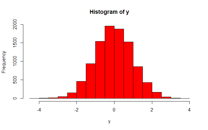
> y <- rnorm(10000)
> hist(y, col="red")