Row and column vectors, and indeterminate vectors A vector, which is interpreted as a row or column vector on the basis of its use, is created by putting the numbers in a list and by using this list as argument of the nparray function. It looks like a row vector, but it is not really the case.

A row vector or column vector is created by putting the numbers in a nested list; this is in fact a matrix with 1 row or 1 column.

Below are, behind the prompts in an interactive Python session, commands to create a vector. A transposed vector is obtained by the method transpose of an nparray object.

>>> np.array([1,2,3]) # vector
array([1, 2, 3])
>>> v = np.array([4, 5, 6]); print(v)      # printout of a vector 
[4 5 6] 
>>> print(v.transpose())                   # transposed vector
[4 5 6]
>>> rv = np.array([[4, 5, 6]]); print(rv)  # row vector 
[[4 5 6]]
>>> cv = np.array([[4], [5], [6]]); print(cv) 
[[4] 
[5] 
[6]] 
>>> cv.transpose()  # transposed columnvector
array([[4, 5, 6]])

Dimension and norm With the shape instruction you can determine whether a vector is a row vector or a column vector. With the size instruction you can determine the length of a vector, i.e., the number of components. So not confuse this with what is understood in mathematics by the (Euclidean) length of a vector, namely the norm. The norm can be calculated numerically in Python with the linear algebra command norm and there are options to calculate variations.

>>> v = np.array([4,5,6])
>>> type(v)
<class 'numpy.ndarray'>
>>> v.shape
(3,)
>>> np.size(v)
3
>>> print(cv)      # column vector 
[[4] 
[5] 
[6]] 
 >>> la.norm(cv)   # Euclidean length
8.774964387392123
>>> la.norm(kv,1)  # sum of absolute values of components
15.0 
>>> la.norm(kv, np.inf) # maximum of absolute values of components
6.0

Special constructions There are also special commands to create specific vectors; we show a few commonly used constructions.

>>> v1 = np.arange(5,11); print(v1)    # from 5 to 10 
[ 5 6 7 8 9 10] 
>>> v2 = np.arange(10,4,-2); print(v2) # from 10 to 4 with steps of -2
[10 8 6]
>>> v3 = np.linspace(0,1,6)  # equidistant distribution of 6 points in [0,1] 
>>> print(v3) 
[0. 0.2 0.4 0.6 0.8 1. ]
>>> v4 = np.zeros((3,1), dtype=int);   # column vector with 3 zeros
>>> print(v4)
[[0]
[0]
[0]]
>>> v5 = np.ones((3,), dtype=bool)     # row vector with logical values 1 
>>> print(v5) 
[ True, True, True] 
>>> v6 = np.array([]); print(v6) 
 []

Concatenating vectors You can create new vectors by concatenating vectors. For this you can use the functions concatenate, hstack and vstack.

>>> v1 = np.arange(1,4); v2 = np.arange(4,7); v12 = np.hstack((v1,v2)) 
>>> print(v12) 
[1 2 3 4 5 6] 
>>> np.concatenate((v1, v2)) 
array([1, 2, 3, 4, 5, 6])

Randomly generated vectors In simulations you can make extensive use of vectors with randomly generated numbers, i.e. ,with random numbers. There are several instructions for this purpose.

>>> np.random.rand(5,1) 
array([[0.60839603], 
[0.08385416], 
[0.18951417], 
[0.0336493 ], 
[0.3009523 ]]) 
>>> # 10 random integers between 5 en 8 (inclusive):
>>> np.random.randint(5, high=9, size=10) 
array([8, 8, 8, 7, 5, 8, 8, 7, 5, 6])
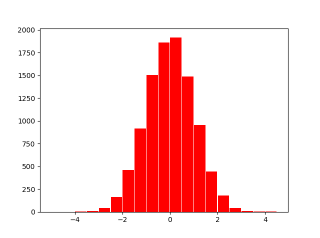
>>> # 5 random numbers generated from the standard normal distribution: 
>>> np.random.standard_normal(5) 
array([-0.48421341, 2.63156996, -0.28340041, -1.55714191, 0.69337535]) 
>>> x = np.arange(-5, 5, 0.5) 
>>> y = np.random.standard_normal(10000) 
>>> import matplotlib.pyplot as plt 
>>> N, bins, patches = plt.hist(y,x,color='r', rwidth=0.95) 
 >>> plt.show()