Linear mappings: Linear mappings
 Kernel and image of a matrix mapping
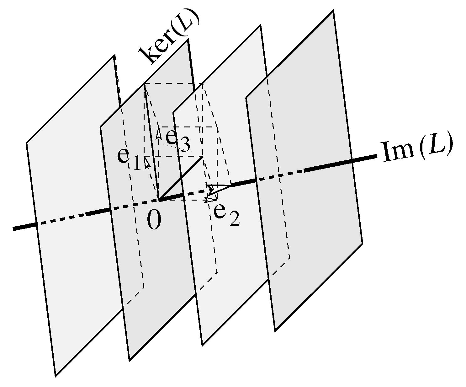
Before we introduce the kernel and image of a linear mapping in formal terms we first have a look at an example in the three-dimensional coordinate space.
Consider the linear mapping \(L: \mathbb{R}^3\longrightarrow \mathbb{R}^3\) defined by \[L\cv{x \\y\\z}=\cv{x-y-z\\ -x+y+z\\-x+y+z}\] This can be rewritten as follows: \[L\cv{x \\y\\z}=x\cv{1\\-1\\-1}+y\cv{-1\\1\\1}+z\cv{-1\\1\\1}=(x-y-z)\cv{1\\-1\\-1}\] The set of all possible images, the image of \(L\), is therefore the line \(\ell\) through the origin with direction vector \(\cv{1\\-1\\-1}\). The set of originals of points on this line, that is to say, all points in space that are mapped to a point on the line \(\ell\), are: \[\begin{aligned} L^{-1}\cv{a\\-a\\-a} &= \left\{\cv{x\\ y\\ z} \middle|\; x-y-z=a\right\} \\ \\ &= \left\{\cv{a+\lambda+\mu\\ \lambda\\ \mu} \middle|\; \lambda, \mu\in\mathbb{R}\right\} \\ \\ &= \cv{a\\ 0\\ 0}+ \lambda\cv{1\\1\\0}+\mu\cv{1\\0\\1}\end{aligned}\] These are parallel planes (each of the planes, which are perpendicular to the direction vector of the line \(\ell\), is mapped to one point).

Only one of these planes passing through the origin, namely, \(L^{-1}(\vec{0})\). This is the kernel of \(L\).
Kernel Let \(A\) be an \(m\times n\) matrix and \(L_A: \mathbb{R}^n\longrightarrow \mathbb{R}^m\) the matrix mapping determined by this matrix. The kernel of \(L_A\), denoted by \(\text{ker}(L_A)\), is the set of vectors in \(\vec{v}\in \mathbb{R}^n\) that are mapped to the null vector. This definition explains the alternative name null space of \(L_A\). As a mathematical formula: \[\text{ker}(L_A)=L_A^{-1}(\vec{0})=\{\vec{v}\in\mathbb{R}^n \mid L_A(\vec{v})=\vec{0}\}\]
Calculation of the kernel The definition of the kernel of a matrix mapping \(L_A\) also suggests the method to compute the null space: consider the matrix \(A\) as the coefficient matrix of a system of linear homogeneous equations. Then the solution set of the system is the kernel of \(L_A\) and this solution set can be found by using the method of Gaussian elimination.
Image Let \(A\) be an \(m\times n\) matrix and \(L_A: \mathbb{R}^n\longrightarrow \mathbb{R}^m\) the matrix mapping determined by this matrix. Each vector \(\vec{v}\in\mathbb{R}^n\) can be written as a linear combination of the unit vectors \(\vec{e}_1, \vec{e}_2, \ldots, \vec{e}_n\). If \[\vec{v}=\lambda_1 \vec{e}_1+ \lambda_2 \vec{e}_2+\cdots+\lambda_n \vec{e}_n\] then \[L_A(\vec{v})=\lambda_1 L_A(\vec{e}_1)+ \lambda_2 L_A(\vec{e}_2)+\cdots+\lambda_n L_A(\vec{e}_n)\] The set of all images of vectors in \(\mathbb{R}^n\) under the matrix mapping, that is, the image of \( L_A\), denoted as \(\text{im}(L_A)\), is thus the linear span of the images of the unit vectors. As a mathematical formula: \[\text{im}(L_A)=\sbspmatrix{L_A(\vec{e}_1),\ldots, L_A(\vec{e}_n)}\] Some authors of mathematics textbook refer to the image of \(L_A\) as the range of the mapping \(L_A\), in order to stay close to the terminology of functions, but we will stick to the more common terms in linear algebra.
Calculation of the image The definition of the image of a matrix mapping \(L_A\) also suggests the method to calculate this: you can compute the linear span of columns of the matrix \(A\) by applying row reduction to the transposed matrix \(A^{\top}\) until the echelon form is obtained and by transposing the intermediate result. The nonzero columns of the in this way obtained columns span the image of \(L_A\).
\[\begin{aligned} \matrix{0&2&0\\0&3&0\\0&-2&0\\}&\sim\matrix{0&1&0\\0&3&0\\0&-2&0\\}&{\blue{\begin{array}{c}{{1}\over{2}}R_1\\\phantom{x}\\\phantom{x}\end{array}}}\\\\ &\sim\matrix{0&1&0\\0&0&0\\0&-2&0\\}&{\blue{\begin{array}{c}\phantom{x}\\R_2-3R_1\\\phantom{x}\end{array}}}\\\\ &\sim\matrix{0&1&0\\0&0&0\\0&0&0\\}&{\blue{\begin{array}{c}\phantom{x}\\\phantom{x}\\R_3+2R_1\end{array}}}\end{aligned}\] We get a matrix with only one nonzero row. This corresponds to the equation \[y=0\] It is a two-dimensional subspace and represents a plane. So \[\text{ker}(L_A)\text{ is the plane with equation }y=0\text.\]
The image of \(L_A\) can be determined by looking at thetransposed of \(A\) and calculate its reduced row echelon form: \[\begin{aligned} \matrix{0&0&0\\2&3&-2\\0&0&0\\}&\sim\matrix{2&3&-2\\0&0&0\\0&0&0\\}&{\blue{\begin{array}{c}R_2\\R_1\\\phantom{x}\end{array}}}\\\\ &\sim\matrix{1&{{3}\over{2}}&-1\\0&0&0\\0&0&0\\}&{\blue{\begin{array}{c}{{1}\over{2}}R_1\\\phantom{x}\\\phantom{x}\end{array}}} \end{aligned}\] in this case we get a matrix with only one nonzero row. The transpose of this is a column vector that spans the image of \(L_A\), which is therefore one-dimensional. So \[ \text{im}(L_A)=\sbspmatrix{\matrix{1 \\ {{3}\over{2}} \\ -1 \\ }}\]
To check the correctness of calculations of the kernel and the image of a matrix mapping you can verify whether your answers satisfy the following dimension theorem, also referred to as the rank theorem or the rank-nullity theorem.
Dimension theorem Consider a matrix mapping \(L_A\) from \(\mathbb{R}^n\) into \(\mathbb{R}^m\) determined by the \(m\times n\) matrix \(A\). Introduce the dimension of the kernel of \(L_A\) as the smallest number of vectors that span the kernel; we denote this number by \(\text{dim}\bigl(\text{ker}(L_A)\bigr)\). The dimension of the null space is also referred as the nullity of the mapping Similarly, we define the dimension of the image of \(L_A\), denoted by \(\text{dim}\bigl(\text{im}(L_A)\bigr)\), as the smallest number of vectors that span \(\text{im}(L_A)\). Then: \[\text{dim}\bigl(\text{im}(L_A)\bigr)+ \text{dim}\bigl(\text{ker}(L_A)\bigr)=n\] The alternative names for the theorem are clear when you write down the following equivalent equality: \[\text{rank}(A)+\text{dim}\bigl(\text{ker}(L_A)\bigr) =n\]


