Transition to a different coordinate system

Linear mappings: Matrices and coordinate transformations

Transition to a different coordinate system

We will generalize the introductory example to the \(n\)-dimensional Euclidean space \(\mathbb{R}^n\).

The unit vectors \(\vec{e}_1=\cv{1\\0\\ \vdots \\ \vdots \\ 0}, \vec{e}_2=\cv{0\\1\\0\\ \vdots \\ 0} \ldots, \vec{e}_n=\cv{0\\ \vdots \\ \vdots \\ 0 \\ 1} \) belong to a choice of a coordinate system in the Euclidean space \(\mathbb{E}^n\). But you can also select a different coordinate system. In fact, you define then axis vectors \(\vec{f}_{\!1}, \vec{f}_{\!2}, \ldots, \vec{f}_{\!n}\) along new axes. Let \[\begin{aligned} \vec{f}_{\!1} &= c_{11}\vec{e}_1+c_{21}\vec{e}_2+\cdots + c_{n1}\vec{e}_n\\ \vec{f}_{\!2}&= c_{12}\vec{e}_1+c_{22}\vec{e}_2+\cdots + c_{n2}\vec{e}_n\\ &\;\;\vdots \\ \vec{f}_{\!n} &= c_{1n}\vec{e}_1+c_{2n}\vec{e}_2+\cdots + c_{nn}\vec{e}_n \end{aligned}\] Then the transformation matrix \([\textit{Id}]_e^f\) is defined by \[[\textit{Id}\,]_e^f=\matrix{c_{11} & c_{12} & \cdots & c_{1n}\\ c_{21} & c_{22} & \cdots & c_{2n} \\ \vdots & \vdots & \ddots & \vdots\\ c_{n1} & c_{n2} & \cdots & c_{nn}}\] Make sure that you take the transformed form of the number scheme in the linear combinations of the \(e\) vectors.

Each vector \(\vec{v}\) in \(\mathbb{E}^n\) can be written as linear combination \([\vec{v}]_e\) of the unit vectors \(\vec{e}_1, \vec{e}_2, \ldots, \vec{e}_n\). We write \[[\vec{v}]_e = \alpha_1\vec{e}_1+\alpha_2\vec{e}_2+\cdots + \alpha_n\vec{e}_n\] We can also do the \(\vec{f}_{\!1}, \vec{f}_{\!2}, \ldots, \vec{f}_{\!n}\) : \[[\vec{v}]_f = \beta_1\vec{f}_{\!1}+\beta_2\vec{f}_{\!2}+\cdots + \beta_n\vec{f}_{\!n}\] Naturally we ask ourselves what connection there is between the \(\alpha\)-s and \(\beta\)-s. Well:

\[\cv{\alpha_1\\ \vdots \\ \alpha_n}= \matrix{c_{11} & \cdots & c_{1n}\\ \vdots & \ddots & \vdots \\ c_{n1} & \cdots & c_{nn}}\!\cv{\beta_1 \\ \vdots\\ \beta_n}\] In short notation: \[[\vec{v}]_e = [\textit{Id}\,]_e^f\,[\vec{v}]_f\]The transformation matrix is be definition invertible and we denote this inverse by \([\textit{Id}\,]_f^e\). In other words \[[\vec{v}]_f = [\textit{Id}\,]_f^e\, [\vec{v}]_e = \left([\textit{Id}\,]_e^f\right)^{-1}[\vec{v}]_e\]

Let \(\vec{v}= \beta_1\vec{f}_{\!1}+\cdots + \beta_n\vec{f}_{\!n}\) and \(\vec{v}= \alpha_1\vec{e}_{1}+\cdots + \alpha_n\vec{e}_{n}\), then \[[\vec{v}]_f =\cv{\beta_1 \\ \vdots\\ \beta_n}\quad\text{and}\quad [\vec{v}]_e\cv{\alpha_{\!1} \\ \vdots\\ \alpha_n}\] Because we can use the transformation matrix \([\textit{Id}\,]_e^f\) to write the \(f\)-vectors as linear combinations of the \(e\)-vectors, we have: \[\begin{aligned} \vec{v} &=\beta_1\vec{f}_{\!1}+\cdots + \beta_n\vec{f}_{n} \\ \\ &= \quad \beta_1(c_{11}\vec{e}_{1}+c_{21}\vec{e}_{2}+\cdots c_{n1}\vec{e}_{n}) \\ &\quad{}+ \beta_2(c_{12}\vec{e}_{1}+c_{22}\vec{e}_{2}+\cdots c_{n2}\vec{e}_n)\\ &{} \quad {}\phantom{xxx}\vdots \\ &\quad {}+\beta_n(c_{1n}\vec{e}_1+c_{2n}\vec{e}_2+\cdots c_{nn}\vec{e}_{n}) \\ \\ &=\quad (\beta_1c_{11}+\beta_2 c_{12}+\cdots+\beta_n c_{1n})\vec{e}_{1} \\ &\quad{}+ (\beta_1 c_{21}+\beta_2 c_{22}+\cdots+\beta_n c_{2n})\vec{e}_{2}\\ &{} \quad {}\phantom{xxx}\vdots \\ &\quad{}+ (\beta_1c_{1n}+\beta_2 c_{2n}+\cdots+\beta_n c_{nn})\vec{e}_{n} \end{aligned}\] Dus: \[\begin{aligned} \alpha_1 &= c_{11}\beta_1+ c_{12}\beta_2+\cdots+ c_{1n}\beta_n \\ \alpha_2 &= c_{21}\beta_1 + c_{22}\beta_2+\cdots+ c_{2n}\beta_n \\ &\vdots \\ \alpha_n &= c_{n1}\beta_1+ c_{n2}\beta_2+\cdots+ c_{nn}\beta_n\end{aligned} \] In matrixvector-vorm staat hier \[\cv{\alpha_1\\ \vdots \\ \alpha_n}= \matrix{c_{11} & \cdots & c_{1n}\\ \vdots & \ddots & \vdots \\ c_{n1} & \cdots & c_{nn}}\!\cv{\beta_1 \\ \vdots\\ \beta_n}\]

Let \(L\) be a linear mapping from \(\mathbb{R}^n\) to \(\mathbb{R}^n\). We already know that it is a matrix mapping when we choose of a coordinate system, that is, that there is a matrix \([A]_e^e\) such that \(L(\vec{v}) = [A]_e^e\,[\vec{v}]_e\). Here we have used the labels \(e\) to indicate the selected coordinate system with corresponding unit vectors \(\vec{e}_1,\ldots, \vec{e}_n\). The same linear mapping \(L\) can also be described with respect to another coordinate system with axis vectors \(\vec{f}_{\!1},\ldots, \vec{f}_{\!n}\) by means of a matrix \([A]_f^f\). The following theorem describes the relationship between the two matrices.

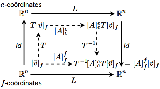
In the transition from \(e\)-coordinates to \(f\)-coordinates applies \[[A]_f^f=[\textit{Id}\,]_f^e\cdot[A]_e^e\cdot[\textit{Id}\,]_e^f\tiny.\] If we abbreviate the transformation matrix \([\textit{Id}\,]_e^f\), which describes the vectors \(\vec{f}_{\!1}, \ldots \vec{f}_{\!n}\) as linear combinations of the vectors \(\vec{e}_1, \ldots, \vec{e}_n\), with the letter \(T\), we have \[[A]_f^f=T^{-1}\cdot [A]_e^e\cdot T\] The diagram below illustrates the coordinate transformation.

For those wondering why we use the label \(e\) twice in the matrix mapping \([A]_e^e\): we do this so that we can also handle coordinate transformations in the case of a linear mapping from \(\mathbb{R}^n\) to \(\mathbb{R}^m\). Suppose that we have chosen in the image space a coordinate system with unit vectors \(\vec{f}_{\!1}, \ldots, \vec{f}_{\!m}\), and suppose that we have chosen in the other space a coordinate system with unit vectors \(\vec{e}_{1}, \ldots, \vec{e}_{n}\), then a linear mapping \(L\) with \[\begin{aligned} L(\vec{e}_{\!1})=a_{11}\vec{f}_{\!1}+a_{12}\vec{f}_{\!2}+\cdots+a_{1m}\vec{f}_{\!m}\\ L(\vec{e}_{\!2})=a_{21}\vec{f}_{\!1}+a_{22}\vec{f}_{\!2}+\cdots+a_{2m}\vec{f}_{\!m}\\ &\vdots \\ L(\vec{e}_{\!n})=a_{n1}\vec{f}_{\!1}+a_{n2}\vec{f}_{\!2}+\cdots+a_{nm}\vec{f}_{\!m}\end{aligned}\] is a matrix mapping with \(m\times n\) matrix \[[A]_e^f=\matrix{a_{11} & \ldots & a_{n1}\\ \vdots & \ddots & \vdots\\ a_{1m} & \ldots & a_{nm}}\] such that each vector \(\vec{v}\) is mapped on \(L(\vec{v})\) via the matrix-vector multiplication \[[L(\vec{v})]_f=[A]_e^f\,[\vec{v}]_e\]

We can also choose different coordinate systems, such \(e'\)- and \(f'\)-coordinates instead \(e\)- and \(f\)-coordinates. Then: \[\begin{aligned} {[A]}_{f'}^{e'} &=[\textit{Id}]_{f'}^{f}\cdot [A]_f^e\cdot [\textit{Id}]_e^{e'} \\ &=\left([\textit{Id}]_{f}^{f'}\right)^{-1}\cdot [A]_f^e\cdot [\textit{Id}]_e^{e'}\end{aligned} \] If we abbreviate the transformation matrix \([\textit{Id}\,]_e^{e'}\) that describes the vectors \(\vec{e}_{1}', \ldots \vec{e}_{n}'\) as linear combinations of the vectors \(\vec{e}_1, \ldots, \vec{e}_n\), with the symbol \(P\), and if abbreviate the transformation matrix \([\textit{Id}\,]_{f}^{f'}\) that describes the vectors (\vec{f}'_{\!1}, \ldots \vec{f}'_{\!m}\) as linear combinations of the vectors \(\vec{f}_{\!1}, \ldots \vec{f}_{\!n}\), with the letter \(Q\), then we have: \[[A]_{e'}^{f'}=Q^{-1}\cdot [A]_f^e\cdot P\]

Let \(L\) be the mapping from \(\mathbb{R}^2\) to \(\mathbb{R}^2\) defined by \[L(x,y)=(2x+y, x-y)\]
What is the matrix \([L]_e^e\) in terms of the unit vectors \(\vec{e}_1=\cv{1\\0}\) and \(\vec{e}_2=\cv{0\\1}\)?

What is the matrix \([L]_f^f\) in \(f\)-coordinates where \(\vec{f}_{\!1}=\matrix{1 \\ -1 \\ }\) and \(\vec{f}_{\!2}=\matrix{-2 \\ 1 \\ }\)?

\([L]_e^e={}\) \(\matrix{2 & 1\\ 1 & -1}\)

\([L]_f^f={}\) \(\matrix{-5 & 9 \\ -3 & 6 \\ }\).

The first equality follows from \[L\cv{1\\ 0}=\cv{2\\1},\quad L\cv{0\\ 1}=\cv{1\\-1}\] by placing these image vectors as columns in the matrix.

The transformation matrix \(T\) from \(f\)-coordinates to \(e\)-coordinates is given by \[T=\matrix{1 & -2 \\ -1 & 1 \\ }\tiny.\] We also need the inverse of this transformation matrix. This can be calculated using the general formula for an inverse \(2\times 2\) matrix, but perhaps better by the below row reduction process \[\begin{aligned}\left(\begin{array}{rr|rr} 1&-2&1&0\\-1&1&0&1\end{array}\right)&\sim\left(\begin{array}{rr|rr} 1&-2&1&0\\0&-1&1&1\end{array}\right)&{\blue{\begin{array}{c}\phantom{x}\\R_2+R_1\end{array}}}\\\\ &\sim\left(\begin{array}{rr|rr} 1&-2&1&0\\0&1&-1&-1\end{array}\right)&{\blue{\begin{array}{c}\phantom{x}\\-R_2\end{array}}}\\\\ &\sim\left(\begin{array}{rr|rr} 1&0&-1&-2\\0&1&-1&-1\end{array}\right)&{\blue{\begin{array}{c}R_1+2R_2\\\phantom{x}\end{array}}}\end{aligned}\] We read: \[T^{-1} = \matrix{-1 & -2 \\ -1 & -1 \\ }\]
Then:
\[\begin{aligned} {[L]}_f^f &=T^{-1}\cdot [L]_e^e \cdot T\\ \\ &= \matrix{-1 & -2 \\ -1 & -1 \\ } \matrix{2 & 1\\ 1 & -1} \matrix{1 & -2 \\ -1 & 1 \\ } \\ \\ &= \matrix{-4 & 1 \\ -3 & 0 \\ } \matrix{1 & -2 \\ -1 & 1 \\ }\\ \\ &=\matrix{-5 & 9 \\ -3 & 6 \\ }\end{aligned}\]

New example