Example 1: linear regression First we calculate the model from the lesson text as follows:

>>> import numpy as np
>>> import numpy.linalg as la
>>> A = np.array([[1,1],[1,2],[1,3]]); print(A) # matrix A for regression line
[[1 1]
 [1 2]
 [1 3]]
>>> b = np.array([2,2,4]);  print(b)            # data vector
[2 2 4]
>>> Ainv = la.pinv(A); print(np.round(Ainv, 4)) # pseudoinverse
[[ 1.3333  0.3333 -0.6667]
 [-0.5     0.      0.5   ]]
>>> print(np.round(Ainv @ b, 4))                # regression coefficients
[0.6667 1. ]     

Actually, the result is in front of your eyes here: \(y= 0.6667+ t\). We can also calculate this outcome via singular value decomposition.

>>> U, S, Vt = la.svd(A, full_matrices=False)   # SVD van A
>>> print(U)                     # matrix U in SVD
[[-0.32310986 0.85377594]
[-0.54750702  0.18321952]
[-0.77190419 -0.4873369 ]]
>>> print(np.diag(S))            # diagonal matrix with singular values
[[4.07914333 0.        ]
 [0.         0.60049122]]
>>> print(Vt)                    # transposed of matrix V in SVD
[[-0.40266324 -0.91534819]
[ 0.91534819 -0.40266324]]
>>> print(U @ np.diag(S) @ Vt)   # check of SVD calculation
[[1., 1.],
 [1., 2.],
 [1., 3.]])
>>> Splus = la.inv(np.diag(S)); print(Splus)
[[0.24514951, 0.        ]
 [0. ,        1.66530329]
>>> Ainv = Vt.transpose() @ Splus @ U.transpose()
>>> print(np.round(Ainv, 4))
[[ 1.3333 0.3333 -0.6667]
 [-0.5    0.     0.5    ]]
>>> print(np.round(Ainv @ b, 4)) # regression coefficients
[0.6667 1. ]      

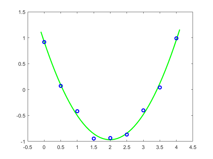
Example 2: quadratic regression The second example is a data set that we create by adding noise to the parabola \(1-2x+\frac{1}{2}x^2\). Hereafter we search for the parabola that fits the created data set best. In our data set this is approximately \(y=0.98-1.94x+0.49x^2\).

>>> import numpy as np
>>> import numpy.linalg as la
>>> import matplotlib.pyplot as plt
>>> x = np.arange(0, 4, 0.5)
>>> y = 1 - 2*x + 1/2*x**2  # parabola
>>> y = y + 0.1*max(y)*(2*np.random.randint(2, size=m) - np.ones(m)) # 10% noise added
>>> A = np.vstack((np.ones(m), x, x**2)).transpose()
>>> pinvA = la.pinv(A)
>>> c = pinvA @ y; print(c)  # pseudoinverse of A gives regression coefficients
[ 0.975 -1.93571429 0.48571429]
>>> xx = np.linspace(-0.1,4.1,50)
>>> yy = c[0] + c[1]*xx + c[2]*xx**2
>>> plt.plot(x, y, 'bo')
>>> plt.plot(xx, yy, 'g-')
>>> plt.axis([-0.1, 4.1, -1.1, 1.1])
>>> plt.show()  # visualisation of data + approximation