Let us carry out in Python a principal component analysis in a concrete example.
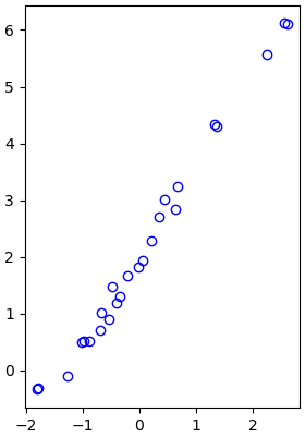
We start with the creation of a data set of two quantities and its visualisation.

>>> import numpy as np
>>> import numpy.linalg as la
>>> import matplotlib.pyplot as plt
>>> X1 = np.random.normal(0, 1, 25)
>>> X1 = np.sort(X1)
>>> X2 = 2 + 1.5*X1 + 0.25*np.random.normal(0, 1, 25) # data on a line + noise
>>> plt.plot(X1, X2, 'bo', mfc='none')
>>> plt.gca().set_aspect('equal')
>>> plt.show()

If we want to do a proper analysis, we first need to edit the data in such a way that the mean values of the two quantities are equal to zero.

>>> X1 = X1 - np.mean(X1)
>>> X2 = X2 - np.mean(X2)
>>> X = np.vstack((X1,X2)))

From the data matrix \(X\) with two quantities (two rows) and \(N=25\) data (25 columns) we can construct the covariance matrix \(C\) as \[C = \frac{1}{N-1}X\,X^{\top}\] Python has for this purpose the function cov in the numpy package.

>>> C = np.cov(X); print(C)
[[1.48630631 2.31901205]
[2.31901205 3.66047268]]

We now want to define new variables whose values are uncorrelated. For this we diagonalise the covariance matrix by solving numerically the eigenvalue problem for the matrix \(C\).

>>> [vals, vecs] = la.eig(C)
>>> print(vals)
[0.01222438 5.13455461]
>>> print(vecs)
[[-0.84393385 -0.53644725]
[ 0.53644725 -0.84393385]]

We sort the eigenvalues in decreasing order and also sort the corresponding eigenvectors.

>>> sorted_index = np.argsort(vals)[::-1]
>>> sorted_vals = vals[sorted_index]
>>> sorted_vecs = vecs[:, sorted_index]

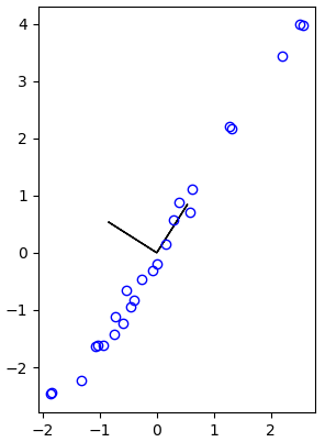
The eigenvectors define new quantities (as linear combinations of the old variables) that are uncorrelated since correlation is nothing else than dotproduct equal to zero for column vectors. In the figure below are shown the two vectors as part of a new coordinate system.

>>> plt.plot(X1, X2, 'bo', mfc='none')
>>> plt.arrow(0,0,-sorted_vecs[0,0],-sorted_vecs[1,0])
>>> plt.arrow(0,0,sorted_vecs[0,1],sorted_vecs[1,1])
>>> plt.gca().set_aspect('equal')
>>> plt.show()

We can transform the data for the new coordinate system and visualise them. Because the eigenvalues are in increasing order, we have to switch columns during the computation.

>>> Y = np.transpose(sorted_vecs) @ X
>>> Y1 = -Y[0,:]  # minus sign for choice of opposite first sorted eigenvector 
>>> Y2 = Y[1,:]
>>> plt.plot(Y1, Y2, 'bo', mfc='none')
[<matplotlib.lines.Line2D object at 0x000001D11480EA90>]
>>> plt.gca().set_aspect('equal')
>>> plt.show()

With the function var we can determine the variation in the quantities. One quantity explains \(99.8\%\) of the variation of the data, and the other quantity only for \(0.2\%\).

>>> varY1 = np.var(Y1); round(varY1, 5)
4.92917
>>> varY2 = np.var(Y2); round(varY2, 5)
0.01174
>>> sumvar = varY1 + varY2
>>> varsY = [varY1/sumvar, varY2/sumvar]; 
>>> print(np.round(varsY, 3))
[0.998 0.002]

\(\phantom{x}\)

We can also use built-in functions for PCA; here we apply pca from the sklearn package and show that we get the same result.

>> from sklearn.decomposition import PCA
>>> pca = PCA(2)
>>> pca.fit(X)
PCA(n_components=2)
>>> pca.fit(np.transpose(X))
PCA(n_components=2)
>>> print(pca.components_) # coefficients of the principal components (factor loadings)
[[ 0.53644725 0.84393385]
[-0.84393385 0.53644725]]
>>> print(pca.explained_variance_)
[5.13455461 0.01222438]
>>> # explained variance along the principal axes
>>> print(np.round(pca.explained_variance_ /sum(pca.explained_variance_), 3))
[0.998 0.002]
>>> YY = pca.transform(np.transpose(X))  # transformed data
>>> round(sum(abs(Y1 - YY[:,0]))) # Y1 = first column of YY
0
>>> round(sum(abs(Y2 - YY[:,1]))) # Y2 = second column of YY
0