MATLAB contains the function svd to determine numerically the singular value decomposition With svds you can compute the six largest singular values (or other specified singular values). First we recalculate the example of the learning material:

>> A = [2 0; 0 -3]
A =
     2     0
     0    -3
>> [U,S,V] = svd(A)  % matrices in SVD
     0     1
     1     0
S =
     3     0
     0     2
V =
     0     1
    -1     0
>> U*S*V' - A   % check
ans =
     0     0
     0     0
>> svds(A)      % largest singular values
ans =
     3
     2

The following example of a singular matrix illustrates the difference between an exact and numerical computation.

$$\begin{aligned}\matrix{1 & -1\\ -1 & 1} &= \matrix{-\frac{1}{2}\sqrt{2} & \frac{1}{2}\sqrt{2} \\ \frac{1}{2}\sqrt{2} & \frac{1}{2}\sqrt{2}}\matrix{2 & 0\\ 0 & 0}\matrix{-\frac{1}{2}\sqrt{2} & \frac{1}{2}\sqrt{2} \\ -\frac{1}{2}\sqrt{2} & -\frac{1}{2}\sqrt{2}}\\ \\ &=\frac{1}{2}\sqrt{2} \matrix{-1 & 1\\ 1 & 1}\matrix{2 & 0\\ 0 & 0}\matrix{-1 & 1\\ -1 & -1}\frac{1}{2}\sqrt{2} \end{aligned}$$

>> B = [1 -1; -1 1]
B =
     1    -1
    -1     1
>> [U,S,V] = svd(B)    % SVD 
U =
   -0.7071    0.7071
    0.7071    0.7071
S =
    2.0000         0
         0    0.0000
V =
   -0.7071   -0.7071
    0.7071   -0.7071
>> U*S*V' - B          % check
ans =
   1.0e-15 *
   -0.3331    0.4441
         0   -0.2220
>> round(ans)          % rounding
ans =
     0     0
     0     0
>> svds(B)             % largest singular values
ans =
2.0000
0.0000

Next comes an example of digital image compression, using a pattern that consists of black and white squares in a $9\times 9$ grid. We specify the figure with a matrix consisting of zeros (white squares) and ones (for black boxes:

$$M = \matrix{ 0 & 0 & 0 & 0 & 1 & 0 & 0 & 0 & 0\\ 0 & 0 & 0 & 1 & 0 & 1 & 0 & 0 & 0 \\ 0 & 0 & 1 & 0 & 0 & 0 & 1 & 0 & 0\\ 0 & 1 & 0 & 1 & 1 &1 & 0 & 1 & 0 \\ 1 & 0 & 0 & 1 & 0 & 1 & 0 & 0 & 1\\ 0 & 1 & 0 & 1 & 1 &1 & 0 & 1 & 0 \\ 0 & 0 & 1 & 0 & 0 & 0 & 1 & 0 & 0\\ 0 & 0 & 0 & 1 & 0 & 1 & 0 & 0 & 0 \\ 0 & 0 & 0 & 0 & 1 & 0 & 0 & 0 & 0}$$ In MATLAB we can visualise this pattern. We specify the figure with a matrix consisting of zeros (white squares) and ones (black squares): $$M = \matrix{ 0 & 0 & 0 & 0 & 1 & 0 & 0 & 0 & 0\\ 0 & 0 & 0 & 1 & 0 & 1 & 0 & 0 & 0 \\ 0 & 0 & 1 & 0 & 0 & 0 & 1 & 0 & 0\\ 0 & 1 & 0 & 1 & 1 &1 & 0 & 1 & 0 \\ 1 & 0 & 0 & 1 & 0 & 1 & 0 & 0 & 1\\ 0 & 1 & 0 & 1 & 1 &1 & 0 & 1 & 0 \\ 0 & 0 & 1 & 0 & 0 & 0 & 1 & 0 & 0\\ 0 & 0 & 0 & 1 & 0 & 1 & 0 & 0 & 0 \\ 0 & 0 & 0 & 0 & 1 & 0 & 0 & 0 & 0}$$ In MATLAB we can visualise this pattern.

>> M = [
0 0 0 0 1 0 0 0 0;
0 0 0 1 0 1 0 0 0;
0 0 1 0 0 0 1 0 0;
0 1 0 1 1 1 0 1 0;
1 0 0 1 0 1 0 0 1;
0 1 0 1 1 1 0 1 0;
0 0 1 0 0 0 1 0 0;
0 0 0 1 0 1 0 0 0;
0 0 0 0 1 0 0 0 0];            % pattern
>> colormap([1 1 1; 0 0 0]);   % specify 2 colours: black and white
>> image(M .* 255);            % pattern as black-and-white figure

Suppose we want to send someone this pattern. Then we can send the matrix $M$, that is. 81 numbers one and zero. But you can send fewer numbers when you use the singular value decomposition, while the image can still be reconstructed.

The eigenvalues of the matrix $M$ are as follows in increasing order:

>> sort(eig(M))
ans =
   -2.0000
   -0.9032
   -0.0000
   -0.0000
   -0.0000
    0.0000
    1.1939
    2.0000
    3.7093

Thus, the singular values of $M$ are in descending order, rounded to 1 decimal place, equal to $3.7$, $2.0$, $1.2$, $0.9$ and $0$.

>> svds(M)
ans =
    3.7093
    2.0000
    2.0000
    1.1939
    0.9032
    0.0000

We approximate $M$ now with the first terms of the singular value decomposition. But instead of using the numerical values of the decomposition for image display we round the elements of the matrix elements to whole numbers $0$ and $1$ to reconstruct the pattern.

Suppose we only use the highest singular value $3.7$. Then the picture looks already a bit like the original figure:

>> [U,S,V] = svd(M);
>> M1 = round(U(:,1)*S(1,1)*V(:,1)'); 
>> image(M1 .* 255)

To do so we only need to transmit $1+2\times 9 = 19$ numeric values, namely the singular value and the two vectors $\vec{u}_1$ and $\vec{v}_1$.

If we also include the singular value $2$, we get even back the original figure.

>> M3 = round(U(:,1:3)*S(1:3,1:3)*V(:,1:3)');
>> image(M3 .* 255)

Now it suffices to transmit $3+6\times 9 = 57$ numerical values, namely $3$ eigenvalues and $2\times 3= 6$ vectors. This does not seem so much less than $81$, it is already a reduction of approximately $30\%$

$\phantom{xx}$

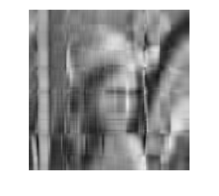
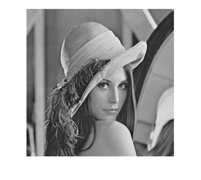
The gain is more spectacular when transmitting large digital images, for example in the picture commonly used in computer vision from $512\times 512$ pixels.

We read the image into the software environment, calculate the singular value decomposition of the corresponding $512\times 512$ matrix with grayscale values, and approximate the original image with 8, 16, 32, 64, and 128 terms from the singular value decomposition.

>> im = imread('E:/ANS/Lena512.bmp');
>> img = im2double(im);
>> size(img)
ans =
   512   512
>> imshow(img)
>> [U,S,V] = svd(img);
>> img8= U(:,1:8)*S(1:8,1:8)*V(:,1:8)';
>> imshow(img8)
>> img16= U(:,1:16)*S(1:16,1:16)*V(:,1:16)';
>> imshow(img16)
>> img32= U(:,1:32)*S(1:32,1:32)*V(:,1:32)';
>> imshow(img32)
>> img64= U(:,1:64)*S(1:64,1:64)*V(:,1:64)';
>> imshow(img64)
>> img128= U(:,1:128)*S(1:128,1:128)*V(:,1:128)';
>> imshow(img128)

Below we present the images for different values of the number of terms $k$ extracted from the SVD. Clearly less information you need while still having a picture that differs on first sight little form the original (at $k=64$ the compression factor is about $\frac{1}{4}$). With colour pictures, the gain is even greater.

$k=8$	$k=16$
$k=32$	$k=64$
$k=128$	Original: $k=512$