Example 1: linear regression First we calculate the model from the lesson text as follows:

>> A = [1 1; 1 2; 1 3] % matrix A for regression line
A =
     1     1
     1     2
     1     3
>> b = [2; 2; 4]       % data vector
b =
     2
     2
     4
Ainv = pinv(A)         % pseudoinverse
Ainv =
    1.3333    0.3333   -0.6667
   -0.5000    0.0000    0.5000
>> Ainv * b            % regression coefficients
ans =
    0.6667
    1.0000

Actually, the result is in front of your eyes here: \(y= 0.6667+ t\). We can also calculate this outcome via singular value decomposition.

>> [U S V] = svd(A)      % SVD
   -0.3231    0.8538    0.4082
   -0.5475    0.1832   -0.8165
   -0.7719   -0.4873    0.4082
S =
    4.0791         0
         0    0.6005
         0         0
V =
   -0.4027    0.9153
   -0.9153   -0.4027
>> Splus = zeros(2,3);
>> Splus(1:2,1:2) = S(1:2,1:2)^(-1) 
Splus =
    0.2451         0         0
         0    1.6653         0
>> Ainv = V * Splus * U' % pseudoinverse
Ainv =
    1.3333    0.3333   -0.6667
   -0.5000    0.0000    0.5000
>> Ainv * b              % regression coefficients
ans =
ans =
    0.6667
    1.0000

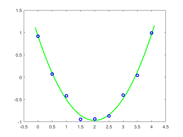
Example 2: quadratic regression The second example is a data set that we create by adding noise to the parabola \(1-2x+\frac{1}{2}x^2\). Hereafter we search for the parabola that fits the created data set best. In our data set this is approximately \(y=0.92-1.90x+0.48x^2\).

>> x = [0:0.5:4]';
>> m = length(x);
>> y = ones(m,1)  - 2*x + x.^2/2;               % parabola
>> y = y + 0.1*max(y)*(2*rand(m,1)-ones(m,1));  % 10 percent noise added
>> A = [ones(m,1) x x.^2 ]
>> pinvA = pinv(A); c = pinvA*y   % pseudoinverse of A gives regression coefficients
c =
    0.9204
   -1.8975
    0.4769
>> xx = linspace(-1.1,1.1,50);
>> yy = c(1)+ c(2)*xx + c(3)*xx.^2;
>> plot(x, y, 'bo', xx, yy, 'g-','LineWidth', 2) % visualisation of data + approximation