Let us carry out in MATLAB a principal component analysis in a concrete example.
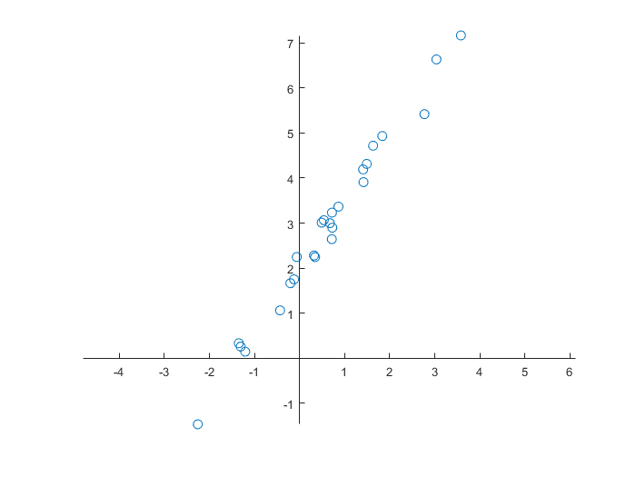
We start with the creation of a data set of two quantities and its visualisation.

>> rng(0);  % control random number generation
>> data(:,1) = randn(25,1);
>> data(:,2) = 2 + 1.5*data(:,1) + 0.25*randn(size(data(:,1))); % data on a line + noise
>> data = sortrows(data,1);  % sort the first column
>> figure
axes('LineWidth',0.6,...
    'FontName','Helvetica',...
    'FontSize',8,...
    'XAxisLocation','Origin',...
    'YAxisLocation','Origin');
line(data(:,1),data(:,2),...
    'LineStyle','None',...
    'Marker','o');
axis equal

If we want to do a proper analysis, we first need to edit the data in such a way that the mean values of the two quantities are equal to zero.

>> data(:,1) = data(:,1)-mean(data(:,1));
>> data(:,2) = data(:,2)-mean(data(:,2));

From the data matrix \(X\) with two quantities (two columns) and \(N=25\) data (25 lines) we can construct the covariance matrix \(C\) as \[C = \frac{1}{N-1}X^{\top}\!X\] MATLAB has for this purpose the function cov on board.

>> C = cov(data)
C =
    1.9179    2.7857
    2.7857    4.1102

We now want to define new variables whose values are uncorrelated. For this we diagonalise the covariance matrix by solving numerically the eigenvalue problem for the matrix \(C\).

>> [V,D] = eig(C)
V =
   -0.8265    0.5630
    0.5630    0.8265
D =
    0.0205         0
         0    6.0076

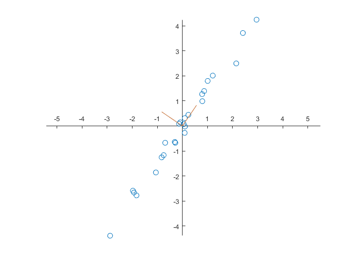
The eigenvectors define new quantities (as linear combinations of the old variables) that are uncorrelated since correlation is nothing else than dotproduct equal to zero for column vectors. In the figure below are shown the two vectors as part of a new coordinate system.

>> figure
axes('LineWidth',0.6,...
    'FontName','Helvetica',...
    'FontSize',8,...
    'XAxisLocation','Origin',...
    'YAxisLocation','Origin');
line(data(:,1),data(:,2),...
    'LineStyle','None',...
    'Marker','o');
line([0 V(1,1)],[0 V(2,1)],...
    'Color',[0.8 0.5 0.3],...
    'LineWidth',0.75);
line([0 V(1,2)],[0 V(2,2)],...
    'Color',[0.8 0.5 0.3],...
    'LineWidth',0.75);
axis equal

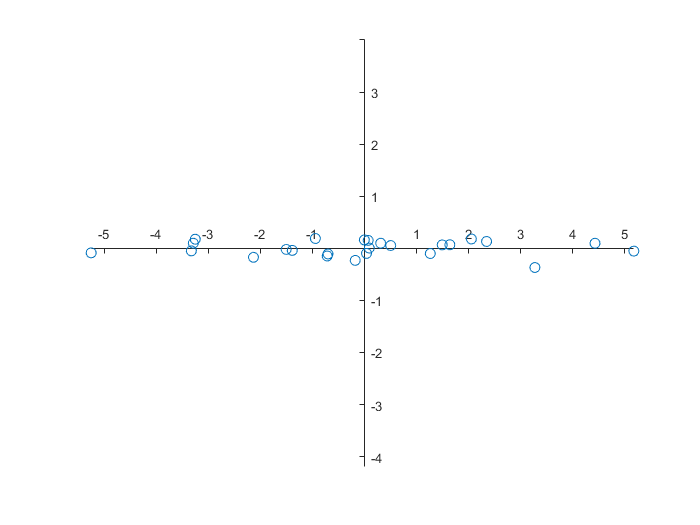
We can transform the data for the new coordinate system and visualise them. Because the eigenvalues are in increasing order, we have to switch columns during the computation.

>> newdata = data * V';
>> newdata = fliplr(newdata)
newdata =
   -5.2475   -0.0866
   -3.2490    0.1749
   -3.2866    0.0982
   -3.3236   -0.0482
   -2.1315   -0.1726
   -1.5034   -0.0214
   -1.3865   -0.0396
   -0.9434    0.1884
   -0.7009   -0.1084
   -0.7160   -0.1476
   -0.0023    0.1615
    0.0702    0.1519
    0.0915    0.0045
   -0.1780   -0.2314
    0.3098    0.0978
    0.0389   -0.0966
    0.5021    0.0535
    1.4919    0.0659
    1.2632   -0.0997
    1.6386    0.0683
    2.0519    0.1797
    2.3433    0.1318
    3.2713   -0.3681
    4.4254    0.0968
    5.1706   -0.0531
>> figure
axes('LineWidth',0.6,...
    'FontName','Helvetica',...
    'FontSize',8,...
    'XAxisLocation','Origin',...
    'YAxisLocation','Origin')
line(newdata(:,1),newdata(:,2),...
    'LineStyle','None',...
    'Marker','o');
axis equal

With the function var we can determine the variation in the quantities. One quantity explains \(99.96\%\) of the variation of the data, and the other quantity only for \(0.34\%\).

>> var(newdata)
ans =
    6.0076    0.0205
>> var(newdata)/sum(var(newdata))
ans =
    0.9966    0.0034

\(\phantom{x}\)

We can also the built-in function pca in MATLAB.

>> [coeff,newdata,latent,tsd,variance] = pca(data);
>> coeff    % coefficients of the principal components (factor loadings)
coeff =
    0.5630    0.8265
    0.8265   -0.5630
>> newdata  % transformed data
newdata =
   -5.2475    0.0866
   -3.2490   -0.1749
   -3.2866   -0.0982
   -3.3236    0.0482
   -2.1315    0.1726
   -1.5034    0.0214
   -1.3865    0.0396
   -0.9434   -0.1884
   -0.7009    0.1084
   -0.7160    0.1476
   -0.0023   -0.1615
    0.0702   -0.1519
    0.0915   -0.0045
   -0.1780    0.2314
    0.3098   -0.0978
    0.0389    0.0966
    0.5021   -0.0535
    1.4919   -0.0659
    1.2632    0.0997
    1.6386   -0.0683
    2.0519   -0.1797
    2.3433   -0.1318
    3.2713    0.3681
    4.4254   -0.0968
    5.1706    0.0531
>> latent   % eigenvalues of the covariance matrix of the data set
latent =
    6.0076
    0.0205
>> variance % variance in data along the principal axes
variance =
   99.6601
    0.3399
>> corrcoef(newdata)
ans =
    1.0000    0.0000
    0.0000    1.0000