We consider the differential equation \[\frac{\dd y}{\dd t}=1-2t y\]

Part 1

In the first part of the task we must plot the slope field of the above differential equation by making use of graphics elements such as line segments. We have written hereto a function called Slopefield_ODE_Order1. The code is shown below. Herein we have chosen to create a meshgrid with the coordinates, but there are alternatives to solve this problem.

function [ output_args ] = Slopefield_ODE_Order1(range_t , range_y , length_lines)
% Slopefield_ODE_Order1 returns the slope field of the differential
% equation y'= 1-2ty for t values in range_t and y values in range_y.
% The ranges must be of the form starting point : step size : terminal point.
% For example Slopefield_ODE_Order1(0:0.1:2 , 0:0.1:2 , 0.1)
% results in the slope field in the area between t = 0 to 2 and 
% y = 0 to 2 in which steps with size 0.1 are taken in both directions.
% The length of the line segments to be drawn is in this case equal to 0.1.

% Making a meshgrid with all t and y values and determining the corresponding slope:
[t,y] = meshgrid(range_t,range_y);
slope = 1 - 2*t.*y;

% Computing the corresponding angle and starting/terminal points  
% with desired length of lineal elements:
angle = atan(slope);
dt = length_lines * cos(angle);
dy = length_lines * sin(angle);
start_t = t + dt;
end_t = t - dt;
start_y = y + dy;
end_y = y - dy;

% Drawing the lineal elements by going through the coordinates in all grids where
% the properties are stored:
figure('Color','White')
title(strcat('Lijnelementenveld bij y',char(39),' = 1 - 2ty'),'Color','Blue')
box on
for row = 1:length(range_y)
   for column = 1:length(range_t)
      curr_start_t =  start_t(column,row);
      curr_end_t =  eind_t(column,row);
      curr_start_y =  start_y(column,row);
      curr_end_y =  eind_y(column,row);
      
      line([curr_start_t,curr_end_t],[curr_start_y,curr_ind_y],'Color','Blue','LineWidth',1)
      hold on
   end
end

% Adding a horizontal and vertical line through the origin
line([xlim],[0,0],'Color','Black','LineWidth',1)
line([0,0],[ylim],'Color','Black','LineWidth',1)

xlabel('t');
ylabel('y');

end

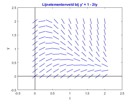
Execution of the command leads to the diagram below.

>> Slopefield_ODE_Order1(0:0.2:2 , 0:0.2:2 , 0.1)

Part 2

In the second part of the task we adapt the program so that \(2000\) random coordinates within the region \(0\le t\le 2, 0\le y\le 2, \) are generated. Hereafter we plot the lineal elements at the points specified by these coordinates. Below is sample code:

function [ output_args ] = Slopefield_ODE_Order1_border(range_t , range_y , length_lines)
% Slopefield_ODE_Order1_border returns the slope field of the differential
% equation y'= 1-2ty for t values in range_t and y values in range_y.
% The ranges must be of the form starting point : step size : terminal point.
% For example Slopefield_ODE_Order1_border(0:2 , 0:2 , 0.1)
% results in the slope field in the area between t = 0 to 2 and 
% y = 0 to 2 in which 2000 random coordinates are chosen.
% The length of the line segments to be drawn is in this case equal to 0.1.

% Creating 2000 random coordinates in the area spanned by range_t and range_y:
t = range_t(1) + (-range_t(1) + range_t(end))*rand(1,2000);
y = range_y(1) + (-range_y(1) + range_y(end))*rand(1,2000);

slope = 1 - 2*t.*y;

% Computing the corresponding angle and starting/terminal point  
% with desired length of lineal elements:
angle = atan(slope);
dt = length_lines * cos(angle);
dy = length_lines * sin(angle);
start_t = t + dt;
end_t = t - dt;
start_y = y + dy;
end_y = y - dy;

% Drawing the lineal elements by going through the coordinate in all grids where
% the properties are stored:
figure('Color','White')
title("Lijnelementenveld bij y' = 1 - 2ty",'Color','Blue')
box on
for coord_no = 1:length(t)
      curr_start_t =  start_t(1,coord_no);
      curr_end_t =  eind_t(1,coord_no);
      curr_start_y =  start_y(1,coord_no);
      curr_end_y =  eind_y(1,coord_no);
      
      line([curr_start_t,curr_end_t],[curr_start_y,curr_end_y],'Color','Blue','LineWidth',1)
      hold on  
end

% Adding a horizontal and vertical line through the origin
line([xlim],[0,0],'Color','Black','LineWidth',1)
line([0,0],[ylim],'Color','Black','LineWidth',1)

end

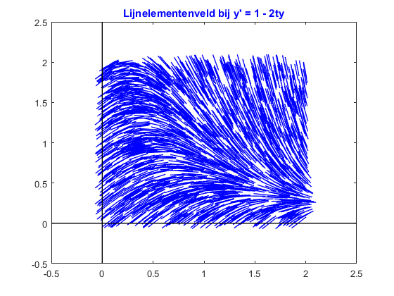
Execution the command leads to the diagram below.

>> Slopefield_ODE_Order1_border(0:2, 0:2, 0.1)