Ordinary differential equations: Slope field and solution curves with Matlab
 Drawing a slope field with the quiver function in MATLAB
Suppose we have a differential equation of the form \[\frac{\dd y}{\dd t} = \varphi(t,y)\] for a certain function \(\varphi\) and we want to draw the slope field using MATLAB. At each point \(t,y\) we can then calculate the slope of a solution \(y\) and draw in the \(ty\)-plane a short line segment with this slope. To do this on a regular grid, the functions meshgrid and quiver are useful.
Basic syntax for slope field, including an example The basic syntax for drawing a slope field in MATLAB is as follows:
[t,y] = meshgrid(tmin:tstep:tmax, ymin:ystep:ymax);
dy = phi(t,y);
dt = ones(size(dy));
figure
quiver(t, y, dt, dy)
In the code line in which dt is set equal to only ones, you can think of writing the differential equation as \[\frac{\dd y}{\dd t} = \frac{\varphi(t,y)}{1}\] A concrete example with \(\varphi(t,y)=1-2\,t\,y\) looks as follows:
>> [t,y] = meshgrid(0:0.12:2, 0:0.1:2);
>> dy = 1 - 2*t.*y;
>> dt = ones(size(dy));
>> figure
>> quiver(t, y, dt, dy);
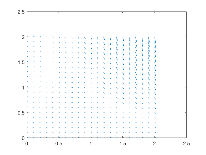
The result is a bit disappointing because the
 quiver function automatically scales the arrows so that they are always visible but the arrows have very different lengths. Also, there is a lot of unnecessary white space above and to the right.
Note that we actually drew a vector field (the default value of quiver) and not a slope field. Also, the starting point of an arrow is in the grid point and we do not put the centre of a vector (or lineal element) on the matching grid point. Via the option ShowArrowHead (default value 'on') we can replace the vectors with segments, but we will not bother about this in the following because the arrows also indicate the direction of a solution curve.
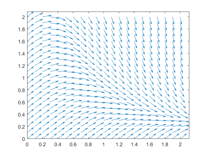
We get the biggest improvement in the slope field by scaling the arrows ourselves so that they all have the same length.
Slope field with scaling of line elements Scaling of the vectors to length 1 can be done in the template via the commands
>> L = sqrt(dt.^2 + dy.^2)
>> dyu = dy./L;
>> dtu = dt./L;
We are now certain that the vectors in \(\cv{dtu\\\ dyu}\) all have length 1. With the axis tight option we remove excess of white space in the slope field. Our earlier example now becomes the following enhanced figure:
>> clear;
>> [t,y] = meshgrid(0:0.1:2, 0:0.1:2);
>> dy = 1 - 2*t.*y;
>> dt = ones(size(dy));
>> L = sqrt(dt.^2 + dy.^2);
>> dyu = dy./L;
>> dtu = dt./L;
>> figure
>> quiver(t, y, dtu, dyu), axis tight
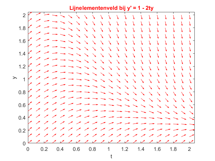
Slope field with different options You can adjust the drawing of the slope field to your liking via options. We give an example in which we reduced the length of the arrows by a scale factor equal to 0.5, chose the colour red, and added labels plus a title.
>> clear;
>> [t,y] = meshgrid(0:0.1:2, 0:0.1:2);
>> dy = 1 - 2*t.*y;
>> dt = ones(size(dy));
>> L = sqrt(dt.^2 + dy.^2);
>> dyu = dy./L;
>> dtu = dt./L;
>> figure
>> quiver(t, y, dtu, dyu, 0.5, 'r'), axis tight
>> xlabel 't', ylabel 'y';
>> title("Lijnelementenveld bij y' = 1 - 2ty",'Color','Red')


