Part 1:

The following is an example of code that implements the forward Euler method for an arbitrary function \(\varphi(t,y)\). We chose to create a main function that calls the Euler function, and in which the plotting is done. This can of course also be done the other way around. In addition, we decided to allow to specify separately what the \(t\) and \(y\) ranges should be for drawing the slope field. Furthermore, additional initial values and the corresponding desired number of steps can be specified in two arrays.

function [ output_args ] = ForwardEulerMethod_Main( ODE, t0, y0, t1, n, 
draw_range_t, draw_range_y, y0_additional, n_additional)
% ForwardEulerMethod_Main draws the slope field of the differential equation 
% specified as ODE and computes a solution curve with initial value (t0,y0) 
% with n steps to t1, via the foward Euler method.
% ODE: if the differential equation is of the form dy/dt = phi(t,y)  
% then the ODE must be of the form 'phi(t,y)'
% t0: time at the initial value y(t0) = y0 of the first solution curve
% y0:  initial value of the first solution curve
% t1:  terminal time for the interval of the solution curves
% n:   the number of steps in the Euler method
% draw_range_t: the interval of the form start_t : step_t : end_t 
% for which the slope field must be drawn.
% draw_range_y: the interval of the form start_y : step_y : end_y 
% for which the slope field must be drawn.
% y0_additional: array of the form [y0_2,y0_3,y0_4,...] with initial values
% for which extra solution curves 
% n_additional: array of the form [n_2,n_3,n_4,...] with corresponding number of
% step for extra solutional curves.
% Example:
% ForwardEulerMethod_Main('1-2.*t.*y',0,2,1,4,0:0.5:2,0:0.5:2,0.1,[],[])
% draws the slope field of the ODE 1-2ty from t = 0 to t = 2 in steps
% of 0.5 and from y = 0 to y = 2 in steps of 0.5. For the solution curve, 
% t0 = 0 and t1 = 1 where n = 4. Thr initial value of y0
% for this solution curve is 2. The length of the linea; elements is 0.1. 
% There asre no extra solution curves to be plotted, so the last two
% parameters are empty arrays.
% The values for eta at each value of t are determined by the function 'Euler':
eta_data = Euler(ODE , t0, y0, t1, n);

% Drawing the slope field together with solution curves. Below we use the
% MATLAB function quiver but yoy could also use a previosly created function 
% that draws the lineal elements
[t,y] = meshgrid(draw_range_t,draw_range_y);
slope = eval(ODE);
angle = atan(slope);
dt = cos(angle); % for own function that draws lineal elements, 
%                  here length_lines*cos(angle) needed.
dy = sin(angle); % for own function that draws lineal elements, 
%                  here length_lines*sin(angle) needed.
figure('Color','White')

% Setting colour and linestyle (the slope field is considered as first object):
set(0,'defaultAxesColorOrder',[1 0 0;0 0 1;1 0 1;0 1 0],
'defaultAxesLineStyleOrder','-|-|--|:') 

% Drawing the slope field. Manual setting of colour because the slope field is expected as first
% object for the colours and line styles specified above. 
quiver(t,y,dt,dy,'Color',[0 114/255 190/255]) 

hold all % later added graphs are involved in the rotation in colour and linestyle. 

% Drawing the foist solution curve. Manual setting of colour because the slope field 
% is expected as first object and the solution curce is otherwise drawn in blue. 
plot(eta_data(1,:),eta_data(2,:),'r','LineWidth',2) 

title(strcat('Lijnelementenveld bij y',char(39),' = ',ODE),'Color','Blue')
xlabel('t')
ylabel('y')
box on
set(gcf,'Color','White')
axis tight

% For multiple solution curves:
no_extra_initial_values = length(y0_additional);
if no_extra_initial_values == 0
    return
else    
    for no = 1:no_extra_initial_values
        y0_no = y0_additional(no);
        n_no = n_additional(no);
        eta_data_extra = Euler(ODE , t0, y0_nr, t1, n_no);        
        plot(eta_data_extra(1,:),eta_data_extra(2,:),'LineWidth',2)

    end
end
end

function [eta_data] = Euler(phi, t0, y0, t1, n)
    % phi: the function in the ODE dy/dt = phi(t,y)
    % t0:  time at the initial value y(t0) = y0 of the first solution curve
    % y0:  initial value of the first solution curve
    % t1:  terminal time for the interval of the solution curves
    % n:   the number of steps in the Euler method
    % OUTPUT: eta_data. This is an array of two sequences. The first sequence
    % contains all points in time and the second sequence contains all
    % computed function values.    
    dt = (t1 - t0) / n ;
    calc_range_t = t0:dt:t1;

    % Initialising a matrix and filling with function values
    eta_prev = y0; % The efirst valuer that must be used for eta_prev.
    eta_data = zeros(2,length(calc_range_t)); % the data matrix filled with zeros.
    eta_data(1,1) = t0; % t0 is now stored in the element with index 1.
    eta_data(2,1) = y0; % y0 is now stored in the element with index 1.
    for k = 2:n+1 % y0,y1,y2, ... are in the array with index 1,2,3,..., respectively
                  % because we let y0 already start at k = 2.
        t = calc_range_t(k-1); % value of t_{k-1}. This is used in eval(phi).
        y = eta_data(2,k-1); % value of eta_{k-1}. This is used in eval(phi).
        eta_data(1,k) = calc_range_t(k);
        eta_data(2,k) = eta_prev + eval(phi)*dt;
        eta_prev = eta_data(2,k); 
    % Store the currently computed value n for reuse in the next step in the repetition.
    end   
end end

The command

>> ForwardEulerMethod_Main('1-2.*t.*y',0,1,2,8,0:0.1:2,0:0.1:2,[1.5],[16])

results in the graph we gave as an example with the assignment:

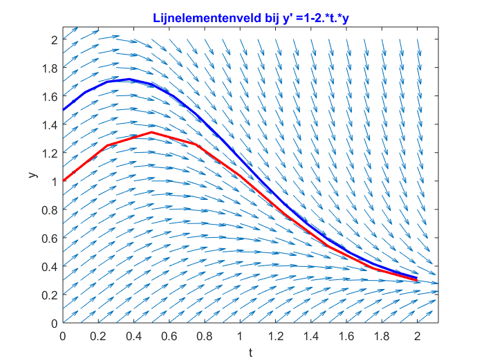
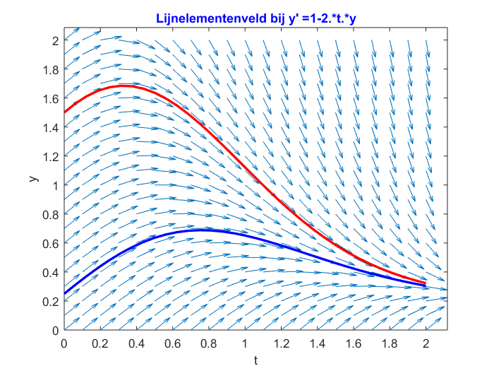
To plot \[\frac{\dd y}{\dd t}=1-2ty,\qquad y(0)=1.5\] and \[\frac{dy}{dt}=1-2ty,\qquad y(0)=.25\] together we enter the following command:

>> ForwardEulerMethod_Main('1-2.*t.*y',0,1.5,2,32,0:0.1:2,0:0.1:2,[0.25],[32])

This results in:

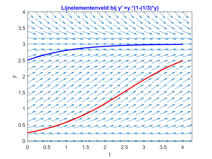
To plot \[\frac{\dd y}{\dd t}=y(1-\tfrac{1}{3}y),\qquad y(-1)=.25\] and \[\frac{dy}{dt}=y(1-\tfrac{1}{3}y),\qquad y(-1)=2.5\] together we enter the following command:

>> ForwardEulerMethod_Main('y.*(1-(1/3)*y)',0,0.25,4,32,0:0.2:4,0:0.2:4,[2.5],[32])

This results in:

Now we can also vary very easily the initial values and the value for \(n\). Below are plotted solution curves of \[\frac{\dd y}{\dd t}=1-2ty\] for the initial values \(0.5\), \(1\), \(1.5\) and \(2\). The corresponding values used for \(n\) are \(4\), \(8\), \(16\) and \(32\). The following command has been used for this:

>> ForwardEulerMethod_Main('y.*(1-2.*t.*y)',0,0.5,2.5,4,0:0.1:2.5,0:0.1:2.5,[1,1.5,2],[8,16,32])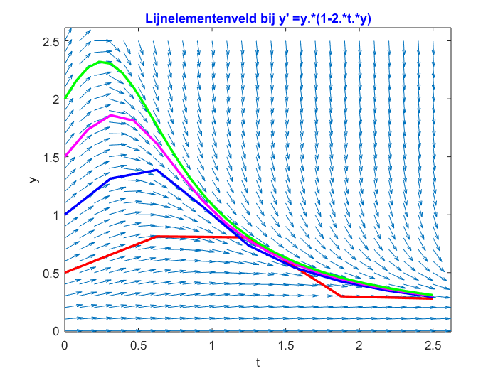

Part 2

For the second part, we use the above function to plot solution curves for several initial values values of (n\) in the same figure. Hereafter we add the result of an 'ode solver' in the command window. A suitable ode solver is ode45 .

The commands you enter might look like this:

>> ForwardEulerMethod_Main('1-2.*t.*y',0,1.5,2,4,0:0.1:2,0:0.1:2,[1.5,1.5,1.5,1.5],[8,16,32,64])
>> [t,y] = ode45(@(t,y) 1-2*t*y,[0,2],1.5);
>> plot(t,y,'k-','LineWidth',2)
>> legend('','n = 4','n = 8','n = 16','n = 32','n = 64','ODE solver')
>> set(0,'defaultAxesColorOrder','remove','defaultAxesLineStyleOrder','remove')

This results in:

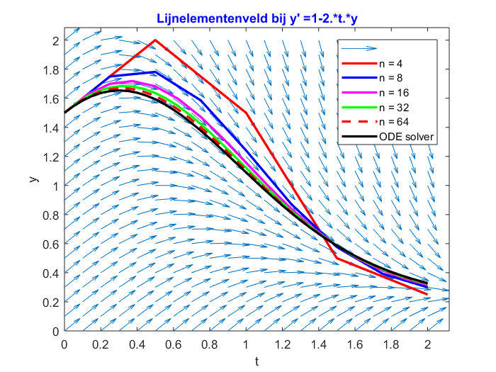
So we see that, as \(n\) bigger, the result of the forward Euler method gets closer and closer to the solution given by the ode solver.