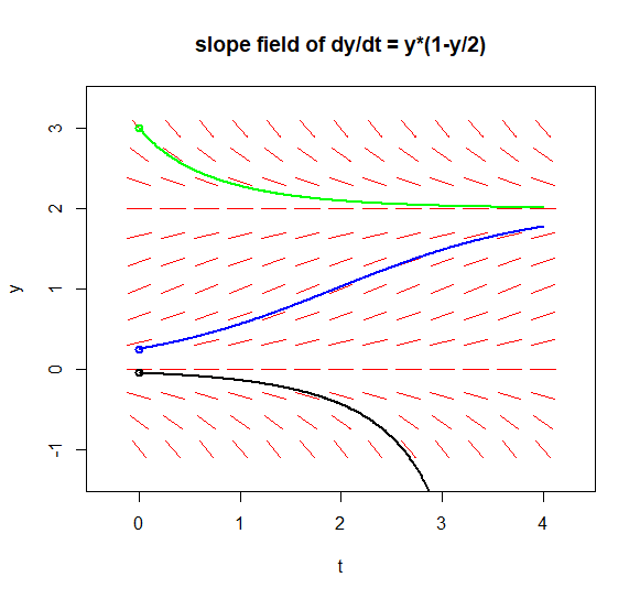
The phaseR package has the flowField function on board to draw the slope field of an autonomous differential equation of order 1 to draw a system of two differential equations. We illustrate the use of the R command by means of the logistic differential equation \[\frac{dy}{dt}=y\cdot (1-y/2)\] In this slop field we also draw three solution trajectory command.

We specify the initial value problem in the code below in the form of an R function with the following three arguments:

• the independent variable, where we usually choose \(t\)
• the initial state of the dependent variable, this being the quantity \(y\);
• parameters, which are parameters \(r\) and \(K\).

The function returns a list of derivatives, but in this case it is just \(\frac{dy}{dt}\), and is used in the numerical method to solve the differential equation. In the code snippet below, the statement with(as.list(c(begintoestand, parameters)). ...) ensures that the names of the parameters are available in the differential equation definition.

library(phaseR)

# Define the ODE
model <- function(time, initialstate, parameters){
  with(as.list(c(initialstate, parameters)), {
    dydt <-  r*y*(1-y/K)
    return(list(dydt))
  })
}

params <- c(r = 1, K = 2) # specify the parameter values

flowField(model, xlim = c(0, 4), ylim = c(-1, 3), 
          parameters = params, system = "one.dim",
          state.names = c("y"), points = 13, 
          arrow.head = 0.001, col = "red",
          add = FALSE, xlab = "t", ylab = "y",  
          main = "slope field of dy/dt = y*(1-y/2)")

trajectory(model, parameters = params, system = "one.dim",
           state.names = c("y"), y0 = c(0.25), tlim = c(0, 4), 
           col = "blue", lwd = 2)
trajectory(model, parameters = params, system = "one.dim",
           state.names = c("y"), y0 = c(3), tlim = c(0, 4), 
           col = "green", lwd = 2)
trajectory(model, parameters = params, system = "one.dim",
           state.names = c("y"), y0 = c(-0.05), tlim = c(0, 4), 
           col = "black", lwd = 2)

The above R code draws a slope field together with three solution curves.

With non-autonomous differential equations you must program the slope field yourself and combine it with graphs of solution curves for initial value problems calculated with the R function ode from the deSolve package.

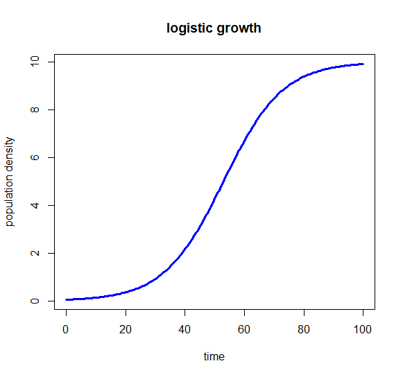
However, as an example of calculating and plotting solution curves, let's look again at the logistic growth model. We look at the initial value \[\frac{dy}{dt}=r\cdot y\cdot (1-y/K), \quad y(0)=y_0\] for \(r=0.1\) and \(K=10\).

As initial value, parameter values, and time interval we successively choose:

library(deSolve)

y0 <- c(y=0.05) # initial value of population density  
params <- c(r=0.1, # relative growth constant r
            K=10)  # carying capacity K
t <- seq(from=0, to=100, by=0.5)  # time interval

The growth model is now solved with the ode command:

solution <- ode(y0, t, model, params)

The output is an object containing an array that tabulates the dependent variable's values at specified times. You can use this to draw a graph of the solution curve. If you want to know more about how the initial value problem is solved numerically, enter the command diagnostics(solution) .

plot(solution, col="blue", main="logistic growth", 
     xlab="time", ylab="population density", lwd=3)

The above R code produces the following diagram: