Existence and uniqueness of solutions

Ordinary differential equations: Slope field and solution curves

Existence and uniqueness of solutions

Given the examples discussed so far, it is perhaps surprising that the domain of a solution plays a role. Indeed, it is not always true that a solution of an initial value problem exists nor that it is alway unique or can be defined for any value of the independent variable.

Mathematicians working in the field of analysis of differential equations ask themselves questions about existence ("Is there at least one solution, and how far in the future and the past?") and uniqueness of initial value problems ("Under what conditions is there at most one solution?"). Thus, for example, the following theorem holds:

Suppose that the functions $\varphi(t,y)$ and $\displaystyle\frac{\partial \varphi(t,y)}{\partial y}$ are continuous on a closed rectangle $R$ in the $ty$ -plane and that $(t_0,y_0)$ is a point within $R$ and not located on an edge of $R$ . Then, the initial value problem

$\frac{dy}{dt}=\varphi(t,y),\quad y(t_0)=y_0$ has a solution $y(t)$ for some $t$ -interval within which $t_0$ is located (existence), but also not more than one solution within the rectangle $R$ at any $t$ interval that contains $t_0$ (uniqueness).

A partial derivative is a concept for functions of several variables. We briefly describe what it means. For a function $f(x,t)$ that depends on location $x$ and time $t$ you can keep one of the variables, say $t$ , constant. Then you get a function in one variable, namely with $x$ as an independent variable. When this function in one variable is a neat function, you can determine its derivative: this derivative is called the partial derivative of $f(x,t)$ with respect to $x$ of order 1, which is denoted as $\dfrac{\partial f(x,t)}{\partial t}$ . You can view the partial derivative as a function of two variables and again compute partial derivatives. Then you get second-order partial derivatives such as:

$\frac{\partial^2 f(x,t)}{\partial x^2}=\frac{\partial}{\partial x}\left(\frac{\partial f(x,t)}{\partial x}\right)\quad\text{and}\quad \frac{\partial^2 f(x,t)}{\partial x \partial t}=\frac{\partial}{\partial x}\left(\frac{\partial f(x,t)}{\partial t}\right)$

The function

$f(x,t)=2x^2+3xt+4t^2$ has the following partial derivatives of order 1 and 2:

$\begin{aligned} \frac{\partial f}{\partial x} &= 4x+3t \\ \\ \frac{\partial f}{\partial t} &= 3x+8t\\ \\ \frac{\partial^2 f}{\partial x^2} &= 4\\ \\ \frac{\partial^2 f}{\partial t^2} &= 8\\ \\ \frac{\partial^2 f}{\partial x\partial t} &= \frac{\partial^2 f}{\partial t\partial x}=3\end{aligned}$

The theorem can be used to define the functions $\mathrm{exp}$ and $\ln$ :

$\mathrm{exp}$ is the unique solution of the intial value problem $\frac{dy}{dt}=y,\quad y(0)=1$ .
$\ln$ is the unique solution of the intial value problem $\frac{dy}{dt}=\frac{1}{t},\quad y(1)=0$ .

If all the details of this theorem are not clear that's not a real problem. In more sloppy words, this theorem states that the initial value problem

$\frac{dy}{dt}=\varphi(t,y),\quad y(t_0)=y_0$ has a unique solution on a certain open interval $I$ with $t_0\in I$ provided that the function $\varphi$ behaves decently near $(t_0,y_0)$ . Such an interval can be chosen to be as large as possible, and then one calls it the maximum existence interval. If the conditions in the above theorem are not fulfilled, then existence and uniqueness can be problematic. Several examples are discussed here:

no solutions of an initial value problem
multiple solutions of an initial value problem
'exploding' solutions and multiple solutions at the price of one formula
solutions that come to a standstill.

No solutions of initial value problem

The initial value problem

$\frac{dy}{dt}=\frac{1}{t},\quad y(0)=0$ has no solution.
The general solution of $\dfrac{dy}{dt}=\frac{1}{t}$ is

$y(t)=\ln\bigl(|t|\bigr)+c$ for some constant $c$ . However, in $t=0$ , this solution is not defined.

The function $t\mapsto \frac{1}{t}$ does not behave properly around $t=0$ ; in fact, it is not even defined for this value. The conditions in the theorem are not met.

Several solutions of an initial value problem

The initial value problem

$\frac{dy}{dt}=\sqrt{y}, \quad y(0)=0$ has two solutions:

$y(t)=t^2\quad\text{and}\quad y(t)=0\text.$

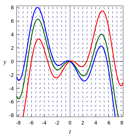
The function $y\mapsto \sqrt{y}$ does not behave properly around $y=0$ ; in fact, it is not even defined for this value. The conditions in the theorem are not met.

Consider the initial value problem

$t \frac{dy}{dt}=y-t^2\cos t,\quad y(0)=0$ There seems nothing to worry about, but rewriting of the initial value problem in the form that is used in the argument for existence and uniqueness

$\frac{dy}{dt}=\frac{y}{t}-t\cos t$ is only possible for $t\neq 0$ . Therefore problems with existence and uniqueness may emerge at $t=0$ . Luckily, this differential equation can be solved exactly and so we can sort out what's going on. First we rewrite the above ODE in the following form:

$\frac{y'\cdot t-y}{t^2}=-\cos t$ Applying the quotient rule for differentiation, one sees on the left-hand side of this equation the derivative of $\displaystyle\frac{y}{t}$ . The right-hand side can be written as the derivative of $-\sin t$ . Thus:

$\left(\frac{y}{t}\right)'=\left(-\sin t\right)'$ The derivatives on the left- and right-hand side of this equation are equal, and thus the functions of which the derivatives are calculated are equal to each other up to a constant. Thus:

$\frac{y}{t}=c-\sin t,$ i.e.

$y=c\,t-t\sin t$ for some constant $c$ . However, for each choice of this constant it holds that $y(0)=0$ . In other words, the initial value problem has infinitely many solutions. Some of the solution curves from this initial value problem are shown in the slope field drawn in the figure below.

multiple solutions

Replace the initial value $y(0)=0$ in the ODE by $y(0)=1$ and the initial value problem has no solution at all.

Blow-up and multiple solutions for the price of one formula

Even when existence and uniqueness are guaranteed, it is still interesting to determine the maximum interval for which the solution of an initial value problem exists. This existence interval often depends on the choice of the initial value. There is actually only local existence: solutions of aninitial value problem need not exist for all time $t$ .

Consider the following initial value problem:

$\frac{dy}{dt}=y^2,\quad y(0)=1$ Then there exists a unique solution

$y=\frac{1}{1-t}$ that "explodes in finite time', namely as $t$ approaches the time $t=1$ . Starting in $t=0$ , the solution curve can be traced infinitely far back in time , but in the forward direction it stops at $t=1$ ; see the figure below. It makes no sense that to consider the part of the graph of $1/(1-t)$ to the right of $t=1$ as a solution curve of the initial value problem. It is, of course, the solution curve of the initial value problem $y'=y^2,\; y(2)=-1.$ In other words, the single formula, $1/(1-t)$ describes in fact two solutions of the ODE $y'=y^2.$

twee exploderende oplossingen

Solutions that come to a standstill

Consider the following differential equation:

$\frac{dy}{dt}=\frac{t+y}{t-y}\tiny.$ The slope field is shown in the figure below, together with some solution curves. What catches the eye is that all solutions are defined over a finite interval, and always go from one edge of the maximum existence interval to the other edge. The solution curves run spirally, counter-clockwise away from a starting point close to the line $y=t$ to another point near this line; in both points is the matching lineal element vertical.

tot stilstand komende oplossingen