Ordinary differential equations: Slope field and solution curves
 'Go with the flow'
A slope field of a differential equation \(\dfrac{\dd y}{\dd t}=\varphi(t, y)\) can give a good impression of how the solution curves look like because these graphs should always touch lineal elements. By drawing a smooth curve for which any point ion the curve is tangent to the lineal element associated with that point you get a so-called integral curve; the graph therefore is a graphical solution of the differential equation. Such a curve has already been referred to as solution curve. We consider two simple examples.
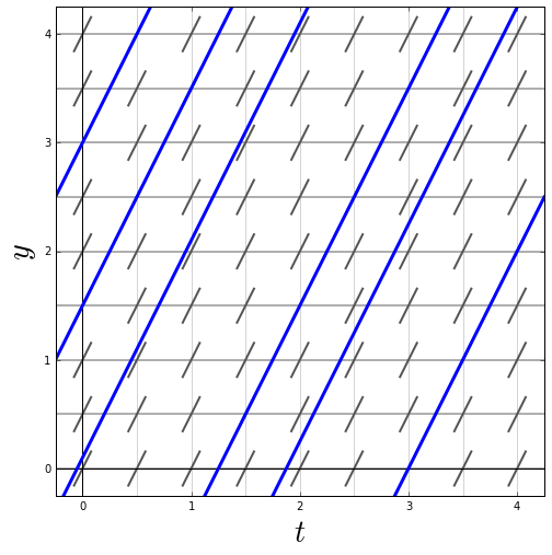
Example 1 We consider the differential equation \[\frac{\dd y}{\dd t}=2\] In the figure below, we added to the slope field graphs of six solutions, namely of \(y=2t+c\) with, from left to right \(c=3, 1.5, 0.1, -2.5, 3.75, -6\). All solutions are line graphs with slope \(1\) because all lineal elements are parallel and have slope \(1\). You can also get a solution of the differential equation by always going in the direction of lineal elements.
Example 2 In the figure below you see on the left-hand side the slope field of the differential equation \[\frac{\dd y}{\dd t}=t\] and on the right-hand side the same slope field but now with graphs of solutions, namely those of \(y=\tfrac{1}{2}t^2+c\) with different values of \(c\). Note that the solution curves always go in the direction of lineal elements; This is what we mean when we write 'go with the flow'.

In this slope field, the isoclines are vertical lines which are steeper when the value \(t\) differs more from \(0\). The nullcline is the vertical axis: this separates lineal elements with negative and positive slopes.


