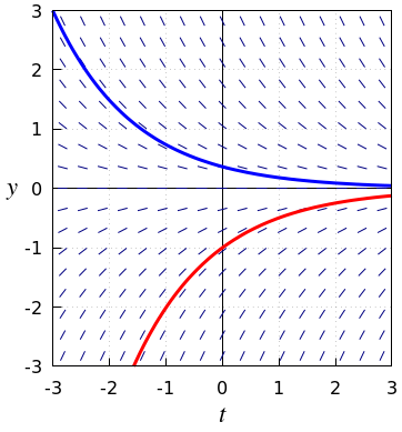
Below is shown a slope field of the differential equation \(\displaystyle\frac{\dd y}{\dd t}=r\cdot y\) with \(r=-0.7\)
(thus \(\varphi(t,y)=-0.7y\) ). It also contains two solution curves in the figure.

The slope field is constructed by drawing at each grid point in the \(ty\)-plane the directional coefficient of the solution as a small, centered line segment with corrsponding slope. The solution for which \(y(2)=1\) has in \(t=2\) a derivative \(y'(2) =r \cdot y(2)=r=-0.7\). Through the point \((2,1)\) we draw therefore a short line segment with slope \(-0.7\). We treat all other grid points in the same way and the line segement are called the lineal elements.

You can play with the below interactive versions of the slope field of any differential equation (in these examples, a differential equation of logistic growth). The first version als containts 'cursor' that can be dragged to any postion to show a corresponding lineal element. There is also shown a solution curve that is determined by the (draggable) red point through which the curve goes.

\(\phantom{abc}\)

An alternative is the interactive version below in which you can plot several solution curves together. Curves can also be removed to shown the lineal elements only.