Worked-out solution We define $$\varphi(y)=y^2+y+b$$ In order to find the equilibria of the differential equation, we must solve the equation$\varphi(y)=0$. This is easy with the $abc$-formula: $$y=\frac{-1\pm\sqrt{1-4b}}{2}$$ There are only real solutions if $1-4b\ge 0$, i.e., if $b\le \tfrac{1}{4}$.

We use local linearisation to determine the nature of the equilibria. Because $\varphi'(y)=2y+1$ we find in the equilibria the values $\pm\sqrt{1-4b}$. It follows, under the condition $b< \tfrac{1}{4}$, that there are two equilibria, of which $y=-\tfrac{1}{2} - \tfrac{1}{2}\sqrt{1-4b}$ is an attractor and $y=-\tfrac{1}{2} + \tfrac{1}{2}\sqrt{1-4b}$ is a repeller. The phase line looks under these conditions as follows:

This result is in agreement with the fact that $\varphi(y)$ is a valley parabola and you can come to the same conclusion by looking at the sign pattern of $\varphi(y)$. If $b= \tfrac{1}{4}$ then we have only a semi-stable equilibrium and the phase line is as follows:

If $b>\tfrac{1}{4}$ then there are no equilibria and the phase line is

In this case there is a saddle-node bifurcation and the bifurcation diagram looks as follows:

Worked-out solution We define $$\varphi(y)=b\cdot y^2+y+1$$ In order to find the equilibria of the differential equation, we must solve the equation $\varphi(y)=0$. This is easy with the $abc$-formula: $$y=\frac{-1\pm\sqrt{1-4b}}{2b}$$ There are only real solutions if $1-4b\ge 0$. i.e., if $b\le \tfrac{1}{4}$ and the case $b=0$ is treated separately, with the equilibrium $y=-1$.

We use local linearisation to determine the nature of the equilibria. Because $\varphi'(y)=2b\cdot y+1$ we find in the equilibria the values $\pm\sqrt{1-4b}$. It follows that there are two equilibria, of which $y=-\tfrac{1}{2b} - \tfrac{1}{2b}\sqrt{1-4b}$ is an attractor and $y=-\tfrac{1}{2b} + \tfrac{1}{2b}\sqrt{1-4b}$ is a repeller. The phase line, in which we indicate the position of the equilibria, looks under the condition $0<b< \tfrac{1}{4}$ as follows:

If $b<0$ then the phase line look as follows:

This result is in agreement with the fact that $\varphi(y)$ is a valley parabola if $b>0$ and a mountain parabola if $b<0$. So, you can come to the same conclusion by looking at the sign pattern of $\varphi(y)$.

If $b=0$ we have one equilibrium, namely $y=-1$, and this is a repeller because then$\varphi'(-1)=1>0$. The phase line is for $b=0$ as follows:

If $b= \tfrac{1}{4}$, then we can rewrite $\varphi(y)$ as $(\tfrac{1}{2}y+1)^2$ and we have only a semi-stable equilibrium, namely $y=-2$. The phase line is now as follows:

If $b>\tfrac{1}{4}$, there are no equilibria anymore and the phase line is

At $b=\tfrac{1}{4}$ we have a saddle-node bifurcation (the number of equilibria changes from 2 to 0).

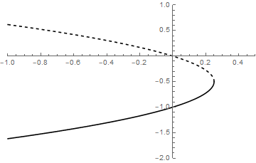
In order to draw the bifurcation diagram correctly you need to figure out where the zeros of $\varphi(y)$ are located for various values of the parameter $b$. A computer generated bifurcation diagram looks as follows:

Worked-out solution We define $$\varphi(y)=b\cdot y^3+y$$ In order to find the equilibria of the differential equation, we must solve the equation $\varphi(y)=0$. This is easiest when you rewrite $\varphi(y)$ as $y\,(b\cdot y^2 +1)$. Then you see that $y=0$ is an equilibrium and that the other equilibria depend on the parameter $b$ because of $b\cdot y^2 + 1=0$. If $b=0$, then there are nu further equilibria. Also, if $b>0$ there are no further equilibria because $b\cdot y^2 + 1$ is in this case a valley parabola with minimum value equal to $1$. If $b<0$ then $b\cdot y^2 + 1$ is a mountain parabola with zeros $y={\pm}1\bigl/\sqrt{|b|}$.

We use local linearisation to determine the nature of the equilibria. Because $\varphi'(y)=3b\cdot y^2+1$ we have $\varphi'(0)=1$ and the equilibrium $y=0$ is a repeller. In addition, we have $\varphi'\Bigl({\pm}1\bigl/\sqrt{|b|}\Bigr)=-2$ and thus the two equilibria $y={\pm}1\bigl/\sqrt{|b|}$ are attractors.

It follows that we only distinguish two kinds of phase lines:

If $b\ge 0$ then

If $b<0$ then

and the attractors move away from each other towards the outside for ascending values of $b$, and they are located closer to each other when $b$ becomes more negative.

The bifurcation diagram looks as follows:

The bifurcation $b=0$ is a supercritical bifurcation because the number of stable equilibria increases when the bifurcation parameter change from positive to negative values.

Worked-out solution We define $$\varphi(y)=y\cdot \left(1-\frac{y}{4}\right)-b$$ In order to find the equilibria of the differential equation, we must solve the equation $\varphi(y)=0$. From the form of the function $\varphi(y)$ we conclude that this is a mountain parabola $y\cdot \left(1-\frac{y}{4}\right)$ that is shifted vertically with $-b$. When we expand the brackets in the polynomial we get $$\varphi(y)= -\tfrac{1}{4}y^2+y-b$$ and the $abc$-formula gives us the zeros $$y=\frac{-1\pm\sqrt{1-b}}{-\tfrac{1}{2}}=2\pm2\sqrt{1-b}$$ provided $b\ge 1$. So there are only equilibria if $b\ge 1$.

If $b=1$ then $\varphi(y)=-(\tfrac{1}{2}y-1)^2$ and it follows from the sign pattern of $\varphi(y)$ that we have a semi-stable equilibrium $y=2$ and a phase line of the form

If $b<1$ then there are two equilibria $y=2\pm 2\sqrt{1-b}$ and because $\varphi(y)$ is a mountain parabola and it follows from the sign pattern of $\varphi(y)$ that $y=2-2\sqrt{1-b}$ is a repelling equilibrium and that $y=2+2\sqrt{1-b}$ is an attractor, and that the phase line looks like

The bifurcation diagram looks as follows:

We have a saddle-node bifurcation at $b=1$.

Worked-out solution We define $$\varphi(y)=b\cdot y-\frac{y}{1+y}$$ In order to find the equilibria of the differential equation, we must solve the equation $\varphi(y)=0$.

If $b=0$ then $$\varphi(y)=-\frac{y}{1+y}$$ and there is an equilibirum $y=0$. In the neighbourhood hereof, the sign pattern of $\varphi(y)$ is equal to the sign pattern of $-y$ and therefore $y=0$ is an attractor.

If $b\neq 0$ then $$\begin{aligned}\varphi(y)=0 &\iff b\cdot y = \frac{y}{1+y}\\\\ &\iff b\cdot y \cdot (1+y) = y \\\\ &\iff y=0\quad\text{of}\quad b\,(1+y)=1 \\ \\ &\iff y=0\quad\text{or}\quad y=\frac{1}{b}-1\end{aligned}$$ So, there are two equilibria. We use local linearisation to determine the nature of the equilibria. First, we compute the following derivative $$\begin{aligned}\frac{\dd \varphi}{\dd y} &= b -\frac{\dd}{\dd y}\left(\frac{y}{1+y}\right) &\blue{\text{sum rule for differentiation}}\\[0.25cm] &= b - \frac{(1+y)-y}{(1+y)^2} &\blue{\text{quotient rule for differentiation}} \\[0.25cm] &= b-\frac{1}{(1+y)^2}\end{aligned}$$ From $\varphi'(0)=b-1$ follows that the equilibrium $y=0$ is attracting if $b<1$, is repelling if $b>1$, and is semi-stable if $b=1$. $$\begin{aligned}\varphi'\left(\frac{1}{b}-1\right) &= b - \frac{1}{\left(\frac{1}{b}\right)^2} \\\\ &= b-b^2 \\\\ &= b\,(1-b)\end{aligned}$$ Because the last term is a mountain parabola in $b$ with zeros at $b=0$ and $b=1$, it follows that the equilibrium $y=\frac{1}{b}-1$ is repelling if $0<b<1$, is semi-stable at $b=1$, and is elsewhere attracting.

We summarize the above stability analysis:

If $b<0$ then there are attractors $y=\frac{1}{b}-1$ and $y=0$, and these are further apart the closer $b$ is to $0$.

If $b=0$ then there exists one equilibrium, namely $y=0$, and it is attracting.

If $0<b<1$ then we have an attractor $y=0$ and a repller $y=\frac{1}{b}-1$.

If $b=1$ then there exists one equilibrium, namely $y=0$, and it is semi-stable.

If $b>1$ then we have a repeller $y=0$ and an attractor $y=\frac{1}{b}-1$e.

The phase lines in the above cases are successively

We have shifted the phase lines in the figure above so that the position of the equilibrium with respect to one another is clearer.

The bifurcation diagram can be sketched or created with mathematical software. It looks like as follows:

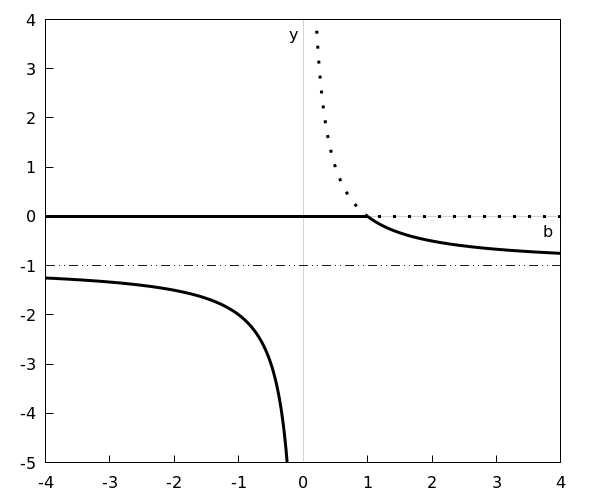
The horizontal blue line represents the line with equation $y=-1$. The bifurcation $b=1$ is a transcritical bifurcation because there is exchange of stability at this point.