For a biological application of stability analysis of a dynamic system and bifurcation, we consider the repetitive outbreaks of the Spruce Budworm population in North American and Canadian coniferous forests. It illustrates how a simple mathematical model can lead to better understanding of the situation and to better measures for handling budworm pests. For details we refer Dutch readers to the accompanying text (in pdf format); below we give a brief summary.

André de Roos & Hans Heesterbeek (2004), Opkomst en ondergang: in de klem tussen bomen en vogels. In H Heesterbeek, O. Diekmann, H. Metz (red.) De wiskundige kat, de biologische muis en de jacht op inzicht. Epsilon Uitgave, Utrecht.

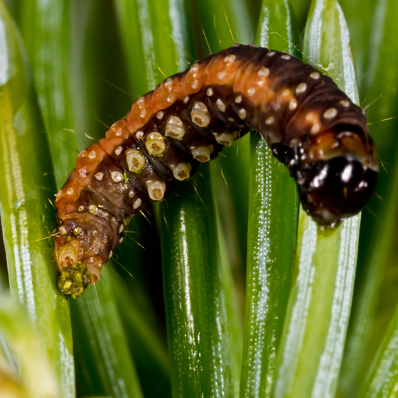
Where in Dutch summers, newspaper in the past decade reported annually about hinder caused by the Oak processionary caterpillar, North American and Canadian newspapers publish for 30 to 40 years alarming news about spruce budworm outbreaks. The budworm is a caterpillar that likes indulging in needles of spruces and therefore causes death to tree in very large parts of forests.

What is going on?

• Normally there are five budworms in a coniferous tree;
• Since the insect outbreak, the number of insects increases in 5-6 yearsto 20,000 per tree;
• The high density of the budworm population causes defoliation and death of trees (9 years after the outbreak);
• After 14 years about 80% of all trees is destroyed;
• The budworm population collapses due to lack of food and predation by birds;
• The forest recovers;
• The phenomenon is repeated.

The economic damage caused by the budworm outbreak causing death of trees in coniferous forests is large regarding tourism and paper industry. For a long time, the main idea was that the outbreaks of the insect population were due to climatic conditions. Using insecticides one tried, in vain, to keep the insect population under control: For example, in 1976 still 400 000 \(\text{km}^2\) was sprayed with insecticides, and in the period from 1952 to 1976 one spent 95 million dollars on insecticides.

A simulation with 30000 parameters was used to select the right management, but only with limited success: forests were back in an 'explosive' situation in 1976. Lucklily science came to the rescue in 1978: a simple mathematical model of Ludwig, Jones and Holling gave an explanation of the cyclical insect outbreaks that destruct large parts of forest. The main conclusion obtained by means of this model was that periodic outbreaks cannot be prevented, but can only be guided in the right direction.

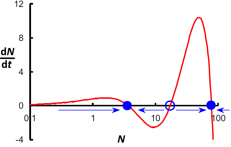
The mathematical model consists of two pieces: a logistic growth model for population growth and a Hill function for population death due to predation by birds in the forest. In mathematical language: \[\frac{\dd N}{\dd t}=r\cdot N\cdot\left(1-\frac{N}{K}\right)- \alpha\frac{N^2}{1+\beta N^2}\] with intrinsic growth coefficient \(r\), carrying capacity \(K\) and positive constants \(\alpha\) and \(\beta\) which determine the maximum predation, as well as the point of inflection in the corresponding predation curve. In the diagram below, \(\dfrac{\dd N}{\dd t}\) is plotted against \(N\) and you can read off that there are two attracting equilibria (at \(N\approx 3\) and \(N\approx 20\)), and a repelling equilibrium (at \(N\approx 10\). All this occurs with the following parameter values \(r=1.2, K=100, \alpha=0.4, \beta=0.02\).

In this model one assumes further that the growth parameters in the logistic part of the model are proportional to the surface area \(A\) of the foliage, say \[r = \gamma\cdot A,\quad K =\frac{\phi}{\gamma}\cdot A\text{.}\] Then: \[\frac{\dd N}{\dd t}=\gamma\cdot A\cdot N-\phi\cdot N^2- \alpha\frac{N^2}{1+\beta N^2}\] We will now explore how the graph of \(\dfrac{\dd N}{\dd t}\) versus \(N\) looks like and this means for the number and kind of equilibria. In the diagram below, these quantities are plotted against each other for various values of \(A\), namely \(A=25,35,45,55,65,75,85\), with \(\gamma= 0.0111, \phi=0.009, \alpha=0.5, \beta=0.1\).

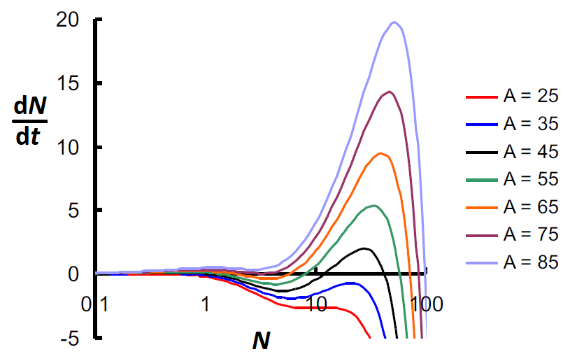
For small values of \(A\) there is only one zero on the left-hand side of the \(N\)-axis and this corresponds with an attracting equilibrium. At very high values of \(A\) there is also only one zero corresponding with an attracting equilibirum. At intermediate values of \(A\) there are 3 zeroes corresponding with two attracting equilibria separated by a repelling equilibrium.

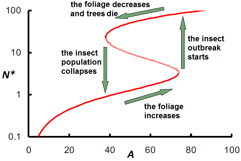
If we take the right-hand side of the differential equation \[\frac{\dd N}{\dd t}=\gamma\cdot A\cdot N-\phi\cdot N^2- \alpha\frac{N^2}{1+\beta N^2}\] and set this term equal to \(0\) in order to find equilibria \(N^{\ast}\), then we can write \(A\) as a function of \(N^{\ast}\): \[A = \frac{\phi\cdot N^{\ast}}{\gamma}-\frac{\alpha}{\gamma}\frac{N^{\ast}}{1+\beta {N^{\ast}}^2}\] We can mirror the graph of this relationship in the diagonal line \(y=x\), so that we get the plot of \(N^{\ast}\) against \(A\). This results in a so-called bifurcation diagram, in which we mark for each parameter value \(A\) attractors by closed circles and the repellers by open circles (or as shown in the figure below as closed and dotted parts of curve, respectively):

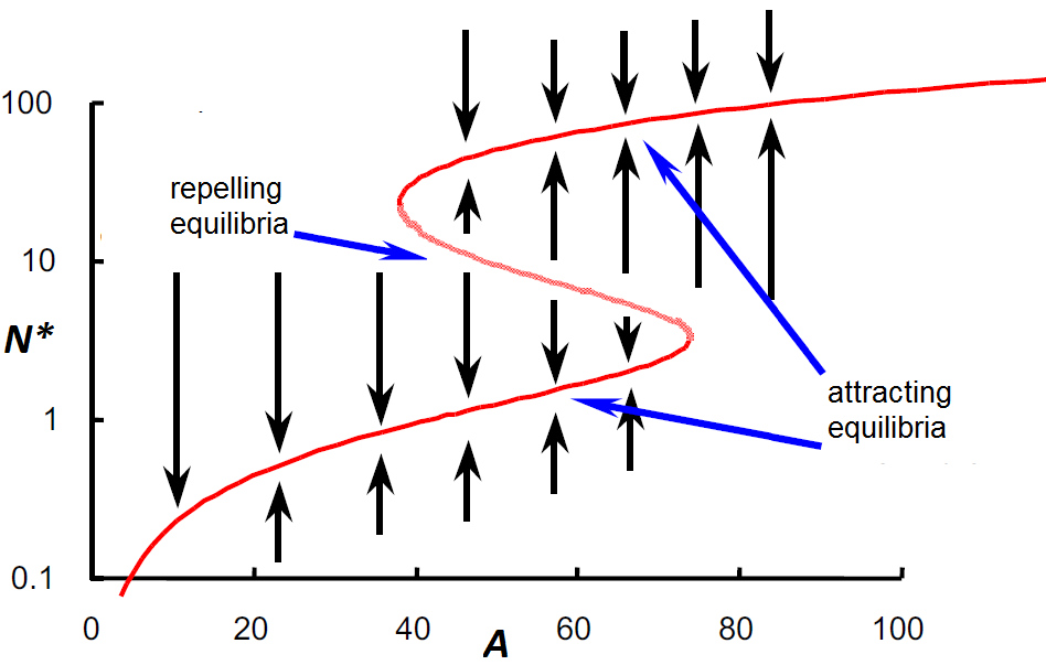
Note that when \(A\) increases and crosses the value \(A\approx 75\) there is all of a sudden only one attracting equilibrium left in the model at a higher value of \(N^{\ast}\). This is the moment of insect outbreak. Similarly, a small decrease around \(A\approx 40\) is sufficient to let the caterpillar population collapse.

The following figure summarizes the scenario of a cyclic insect outbreak and collapse. The outbreak and collapse of the spruce budworm population correspond with the so-called tipping points in the bifurcation diagram.