Fourier series: The Fourier series of an arbitrary function
 Periodic functions with an arbitrary period
Until now, our periodic functions always had a period of \(2\pi\), i.e., we only considered functions \(f(x)\) with the property that \(f(x+2\pi)=f(x)\) all \(x\). We could then concentrate on one period and always chose the interval \((-\pi,\pi)\) for this.
But we generally have to deal with any period \(T\), i.e., with functions for which it is true that \(f(x+T)=f(x)\) for all \(x\). The good news is that we can approximate these functions with sines and cosines as well. This is done as follows: we can define for any given periodic function \(f(x)\) with period \(T\) a new function \(g(x)\) by \[g(x)=f\left(\frac{Tx}{2\pi}\right)\] Then: \[g(x+2\pi) = f\left(\frac{T(x+2\pi)}{2\pi}\right) = f\left(\frac{Tx}{2\pi}+T\right)= f\left(\frac{Tx}{2\pi}\right)=g(x)\] The function \(g(x)\) is periodic with period \(2\pi\) and we already know how to approximate such a function with a Fourier series (at least when Dirichlet's conditions are met, i.e. when the function \(f\) is 'neat'): \[g(x) = a_0+\sum_{n=1}^{\infty}\bigl(a_n\cos(nx) +b_n\sin(n x)\bigr)\] The Fourier coefficients can be calculated with the following formulas \[\begin{aligned} a_0 &= \frac{1}{2\pi}\int_{-\pi}^{\pi}g(x)\,\dd x \\ \\ a_n &= \frac{1}{\pi}\int_{-\pi}^{\pi}g(x)\cos(nx)\,\dd x\qquad\text{if }n\ge 1\\ \\ b_n &= \frac{1}{\pi}\int_{-\pi}^{\pi}g(x)\sin(nx)\,\dd x \qquad\text{if }n\ge 1\end{aligned}\] But then we can also determine the Fourier approximation of the original function \(f(x)\) because \(g(x)=f\left(\frac{Tx}{2\pi}\right)\) can be rewritten as \(f(x)=g\left(\frac{2\pi x}{T}\right)\).
For a 'neat' periodic function \(f(x)\) with period \(T\) we have: \[\begin{aligned}f(x) &= a_0+a_1\cos\left(\frac{2\pi x}{T}\right)+b_1\sin\left(\frac{2\pi x}{T}\right)+ a_2\cos\left(\frac{4\pi x}{T}\right)+b_2\sin\left(\frac{4\pi x}{T}\right)+\ldots\\ \\ &= a_0+\sum_{n=1}^{\infty}\left(a_n\cos\left(\frac{2n\pi x}{T}\right) +b_n\sin\left(\frac{2n\pi x}{T}\right)\right)\end{aligned}\] where the Fourier coefficients can be calculated with the following formulas: \[\begin{aligned} a_0 &= \frac{1}{T}\int_{-\frac{T}{2}}^{\frac{T}{2}}f(x)\,\dd x \\ \\ a_n &= \frac{2}{T}\int_{-\frac{T}{2}}^{\frac{T}{2}}f(x)\cos\left(\frac{2n\pi x}{T}\right)\,\dd x\qquad\text{if }n\ge 1\\ \\ b_n &= \frac{2}{T}\int_{-\frac{T}{2}}^{\frac{T}{2}}f(x)\sin\left(\frac{2n\pi x}{T}\right)\,\dd x \qquad\text{if }n\ge 1\end{aligned}\]
In the above formula of a Fourier approximation there are very many fraction. By a slightly different choice of symbols you can make the formula simpler and more compact. We give the following expression that you may encounter in many textbooks:
For a 'neat' periodic function \(f(x)\) with period \(2L\) we have: \[\begin{aligned}f(x) &= \frac{a_0}{2}+a_1\cos\left(\frac{\pi x}{L}\right)+b_1\sin\left(\frac{\pi x}{L}\right)+ a_2\cos\left(\frac{2\pi x}{L}\right)+b_2\sin\left(\frac{2\pi x}{L}\right)+\ldots\\ \\ &= \frac{a_0}{2}+\sum_{n=1}^{\infty}\left(a_n\cos\left(\frac{n\pi x}{L}\right) +b_n\sin\left(\frac{n\pi x}{L}\right)\right)\end{aligned}\] where the Fourier coefficients can be calculated with the following formulas: \[\begin{aligned} a_n &= \frac{1}{L}\int_{-L}^{L}f(x)\cos\left(\frac{n\pi x}{L}\right)\,\dd x\qquad\text{if }n=0,1,2,\ldots\\ \\ b_n &= \frac{1}{L}\int_{-L}^{L}f(x)\sin\left(\frac{n\pi x}{L}\right)\,\dd x \qquad\text{if }n=1,2,3,\ldots\end{aligned}\]
Consider the function \(f(x)=x^2\) on the interval \((-1,1)\) and continuate it periodically. Then we have: \[f(x)=\frac{1}{3}+\frac{4}{\pi^2}\sum_{n=1}^{\infty} (-1)^n\frac{\cos(n\pi x)}{n^2}\] In this example, the period is equal to 2 (and thus \(L=1\) in the above formulas). So \[f(x)=\frac{a_0}{2}+\sum_{n=1}^{\infty}\bigl(a_n\cos(n\pi x) +b_n\sin(n\pi x)\bigr)\] where \[\begin{aligned} a_0 &= \int_{-1}^{1}x^2\,\dd x = \Bigl[\frac{1}{3}x^3\Bigr]_{-1}^{1} = \frac{2}{3} \\ \\ \\ a_n &= \int_{-1}^{1}x^2\cos(n\pi x)\,\dd x \\ \\ &= \Bigl[\frac{x^2\sin(n\pi x)}{n\pi}\Bigl]_{-1}^{1}-\frac{1}{n\pi}\int_{-1}^{1}x\sin(n\pi x)\,\dd x\qquad\blue{\text{partial integration}} \\ \\ &= \frac{1}{n\pi}\int_{-1}^{1}-x\sin(n\pi x)\,\dd x \\ \\ &= \frac{1}{(n\pi)^2}\cdot \Bigl[x\cos(n\pi x)\Bigr]_{-1}^{1} + \frac{1}{(n\pi)^2} \int_{-1}^{1}\cos(n\pi x)\,\dd x \qquad\blue{\text{partial integration}}\\ \\ &= \frac{4\cos(n\pi)}{(n\pi)^2} +\frac{1}{(n\pi)^3}\Bigl[\sin(n\pi x)\Bigr]_{-1}^{1} \\ \\ &= \frac{4 (-1)^n}{\pi^2n^2}\qquad\text{if }n=1,2,\ldots\\ \\ \\ b_n &= \int_{-1}^{1}x^2\sin(n\pi x)\,\dd x = 0 \qquad\text{if }n=1,2,3,\ldots\\ &\hspace{7.05cm}\blue{\text{ because the integrand is an odd function}}\end{aligned}\] In calculating the latter integral we have used the fact that \[ \int_{-a}^{a} g(x)\,\dd x =0\qquad\text{for an odd function }g(x)\tiny,\] that is, for a function with the property that \(g(-x)=-g(x)\). In this case we have: \[\begin{aligned} \int_{-a}^{a} g(x)\,\dd x &= \int_{-a}^{0} g(x)\,\dd x + \int_{0}^{a} g(x)\,\dd x \\ \\ &= -\int_{a}^{0} g(-y)\,\dd y + \int_{0}^{a} g(x)\,\dd x \\ \\ &= \int_{a}^{0} g(y)\,\dd y + \int_{0}^{a} g(x)\,\dd x\\ \\&= -\int_{0}^{a} g(y)\,\dd y + \int_{0}^{a} g(x)\,\dd x = 0\end{aligned}\] This argumentation we could have used previously when calculating definite integrals.
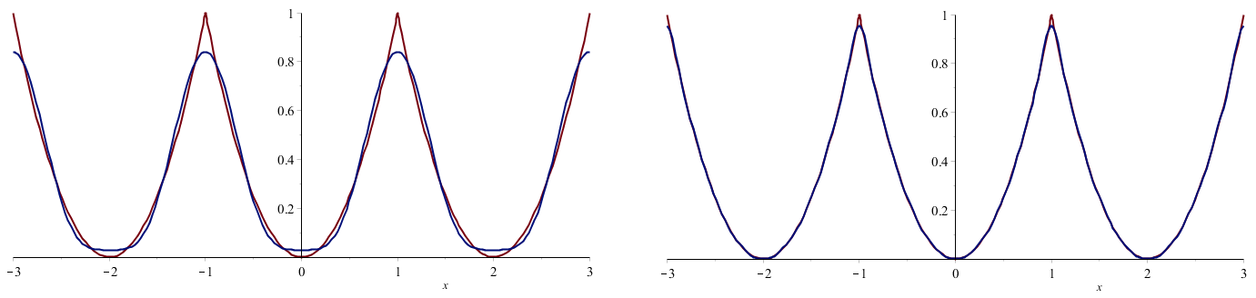
We thus have found the following Fourier series: \[f(x) = \frac{1}{3}+\frac{4}{\pi^2}\sum_{n=1}^{\infty} (-1)^n\frac{\cos(n\pi x)}{n^2}\] In the figure below are shown the graphs of the function and the Fourier cosine series with 2 and 8 cosine terms, respectively. So you have a good approximation.
You can also use the interactive version below to get an impression of how well the function is approximated by a Fourier series and what the frequency-amplitude spectrum looks like.
Substitution of \(x=1\) in the Fourier series leads to: \[ 1 = \frac{1}{3}+\frac{4}{\pi^2}\sum_{n=1}^{\infty} \frac{1}{n^2}\] This can be traced to the following famous formula of Euler: \[\sum_{n=1}^{\infty} \frac{1}{n^2} =\frac{\pi^2}{6}\]