Functions of several variables: Critical points
 Criteria for maximum, minimum, and saddle point
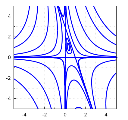
The figure below illustrates the existence of local maxima, local minima, and saddle points for functions of two variables.

As with functions of one variable we want to have efficient criteria to determine the nature of a critical point. For this we look at the second order Taylor approximation of \(f(x,y)\) at a critical point \((a,b)\). For a neat function \(f(x,y)\) of two variables \(x\) and \(y\) we have already seen that we can approximate function values near the point \((x,y)=(a,b)\) via \[\begin{aligned}f(x,y) &\approx f(a,b)+f_x(a,b){\vartriangle}x+f_y(a,b){\vartriangle}y\\ &\phantom{=}+ \frac{1}{2}\!\!\left(f_{xx}(a,b){\vartriangle}x^2+2f_{xy}(a,b){\vartriangle}x{\vartriangle}y+f_{yy}(a,b){\vartriangle}y^2\right)\end{aligned}\] with \[{\vartriangle}x=x-a\quad\text{and}\quad {\vartriangle}y=y-b\tiny.\] When the point \((a,b)\) is a critical point it simplifies to \[f(x,y) \approx f(a,b)+ \frac{1}{2}\!\!\left(f_{xx}(a,b){\vartriangle}x^2+2f_{xy}(a,b){\vartriangle}x{\vartriangle}y+f_{yy}(a,b){\vartriangle}y^2\right)\]
The behaviour of the second order Taylor approximation of \(f(x,y)\) at the critical point \((a,b)\) is thus determined by the quadratic function \[h({\vartriangle}x, {\vartriangle}y)=f_{xx}(a,b){\vartriangle}x^2+2f_{xy}(a,b){\vartriangle}x{\vartriangle}y+f_{yy}(a,b){\vartriangle}y^2\]
- If \(h({\vartriangle}x,{\vartriangle}y)\) has outside \((0,0)\) only positive values, then \((a,b)\) is a local minimum of the function \(f(x,y)\).
- If \(h({\vartriangle}x,{\vartriangle}y)\) has outside \((0,0)\) only negative values, then \((a,b)\) is a local maximum of the function \(f(x,y)\).
- If \(h({\vartriangle}x,{\vartriangle}y)\) has outside \((0,0)\) both positive and negative values, the function \(f(x,y)\) has a saddle point at \((a,b)\).
The range of possible values of \(h(x,y)\) is closely related to the determinant of the Hesse matrix defined as \[\text{Hesse matrix van }f(x,y) = \left(\begin{array}{cc} f_{xx} & f_{xy} \\ f_{xy} & f_{yy}\end{array}\right)\] and evaluated in \((a,b)\). The determinant of the Hesse matrix is called the disciminant or the Hessian of \({f(x,y)}\). We denote \[H(x,y)=f_{xx}(x,y)\cdot f_{yy}(x,y)-f_{xy}(x,y)^2\] and the relationship with \(h({\vartriangle}x,{\vartriangle}y)\) is (after completing the square) \[h({\vartriangle}x,{\vartriangle}y) = \frac{1}{f_{xx}(a,b)}\biggl((f_{xx}(a,b){\vartriangle}x+f_{xy}(a,b){\vartriangle}y)^2+{\vartriangle}y^2\cdot H(a,b)\biggr)\] We can deduce the following criterion:
Second Partial derivatives test for a local maximum, minimum, or saddle point For a neat function \(f(x,y)\) and a critical point \((a,b)\) we have:
- If \(H(a,b)>0\) and \(f_{xx}(a,b)>0\), then \((a,b)\) is a local minimum of the function \(f(x,y)\).
- If \(H(a,b)>0\) and \(f_{xx}(a,b)<0\), then \((a,b)\) is a local maximum of the function \(f(x,y)\).
- If \(H(a,b)<0\), the function \(f(x,y)\) has a saddle point \((a,b)\).
where \[H(a,b)=\det\left(\begin{array}{cc} f_{xx}(a,b) & f_{xy}(a,b) \\ f_{xy}(a,b) & f_{yy}(a,b)\end{array}\right) = f_{xx}(a,b)\cdot f_{yy}(a,b)-f_{xy}(a,b)^2\]
We consider the function\[f(x,y)=3x^2y+xy^2-3xy\] The first partial derivatives are \[f_x(x,y)=6xy+y^2-3y\qquad\text{and}\qquad f_y(x,y)=3x^2+2xy-3x\] The critical points are the solutions of the system of equations \[\left\{\begin{aligned} 6xy+\phantom{2}y^2-3y&=0\\ 3x^2+2xy-3x&=0\end{aligned}\right.\] We have solved this problem before: there are four critical points, namely \((0,0)\), \((1,0)\), \((0,3)\) and \((\tfrac{1}{3},1)\). We now look at the nature of these critical points.
We fist calculate the second partial derivatives: \[f_{xx}(x,y)=6y,\qquad f_{xy}(x,y)=6x+2y-3,\qquad f_{yy}(x,y)=2x.\] Via the scheme below we can make statements about the critical points \[\begin{array}{|c|c|c|c|c|c|} \hline (a,b) & f_{xx}(a,b) & f_{xy}(a,b) & f_{xy}(a,b) & H(a,b) & \textit{conclusion} \\ \hline (0,0) & 0 & -3 & 0 & -9 & \text{saddle point} \\ \hline (1,0) & 0 & 3 & 2 & -9 & \text{saddle point}\\ \hline (0,3) & 18 & 3 & 0 & -9 & \text{saddle point}\\ \hline (\tfrac{1}{3},1) & 6 & 1 & \tfrac{2}{3} & 3 & \text{minimum}\\ \hline \end{array}\]
Contour curves near the critical points have been drawn in the contour graph below. The pattern of closed curves around a critical point (around \((\tfrac{1}{3},1)\) in this example) is typical for a local maximum or minimum. A crossing of curves in a critical point (in \((0,-0), (1,0), (0,3)\) in this example) is typical for a saddle point. You also see often in those points that curves bend away in another direction.

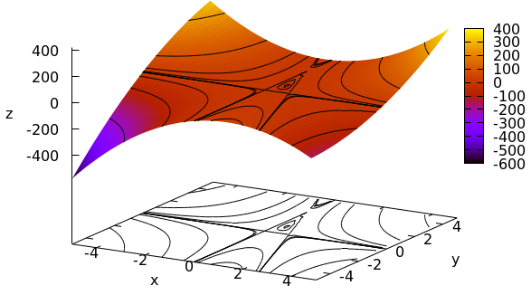
The below computer generated graph of the function with level curves projected on a plane illustrate the analysis (even though the level curves are not so neat due to numerical rounding).


