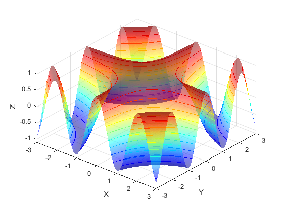
We use the function \[z=f(x,y)=\cos(xy)\] for an example of constructing a contour plot.

We first make the surface graph of the function with some level curves hereon that are made visible through the contour command. In order to obtain a better image we specify a viewing direction with the view command, and we made the surface transparent so that the level curves are well visible. As color image we use a preset scheme in which a low \(z\) value is in the 'cool' colour blue and a high \(z\) value is in the 'warm' colour red.

>> x = linspace(-3,3,500); 
>> y = linspace(-3,3,500); 
>> [x,y] = meshgrid(x,y); 
>> z = cos(x.*y); 
>> fig = figure('Color','White'); 
>> ax = fig.CurrentAxes; 
>> surf(x,y,z,'EdgeColor','none','FaceAlpha',0.5) 
>> colormap(jet) 
>> hold on 
>> contour3(x,y,z) 
>> xlabel('X') 
>> ylabel('Y') 
>> zlabel('Z') 
>> xlim([-3,3]) 
>> ylim([-3,3]) 
>> zlim([-1.1,1.1]) 
>> view(40,45)

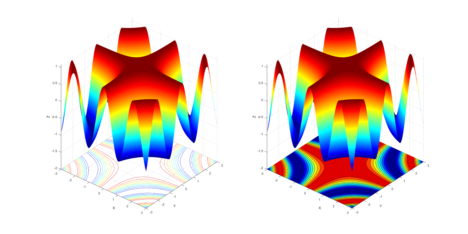
In a contour plot, one projects the level curves on the \(xy\)-plane. Below this is done in two ways, namely with and without filling the space between the level lines. The difference is in the call of contour and contourf, respectively. For clarity we have selected the projection plane \(z=-2\).

>> x = linspace(-3,3,500); 
>> y = linspace(-3,3,500); 
>> [x,y] = meshgrid(x,y); 
>> z = cos(x.*y); 
>> fig = figure('Color','White'); 
>> ax1 = subplot(1,2,1); 
>> h1 = surf(x,y,z,'EdgeColor','None','Parent',ax1); 
>> colormap(jet) >> shading interp 
>> hold on
 >> contour_level = -2; 
>> [ ~,properties] = contour(x,y,z);
>> properties.ContourZLevel = contour_level; % the z positie van de contour instellen
>> view(40,30)
>> xlabel('X')
>> ylabel('Y')
>> zlabel('Z')
>> xlim([-3,3])
>> ylim([-3,3])
>> zlim([contour_level,1.1])
>> ax2 = subplot(1,2,2);
>> h2 = surf(x,y,z,'EdgeColor','None','Parent',ax2);
>> colormap(jet)
>> shading interp
>> hold on
>> contour_level2 = -2;
>> [~ ,properties2] = contourf(x,y,z); >> properties2.ContourZLevel = contour_level; % set the z position of the contour curves 
>> view(40,30) 
>> xlabel('X') 
>> ylabel('Y') 
>> zlabel('Z') 
>> xlim([-3,3]) 
>> ylim([-3,3]) 
>> zlim([contour_level2,1.1])

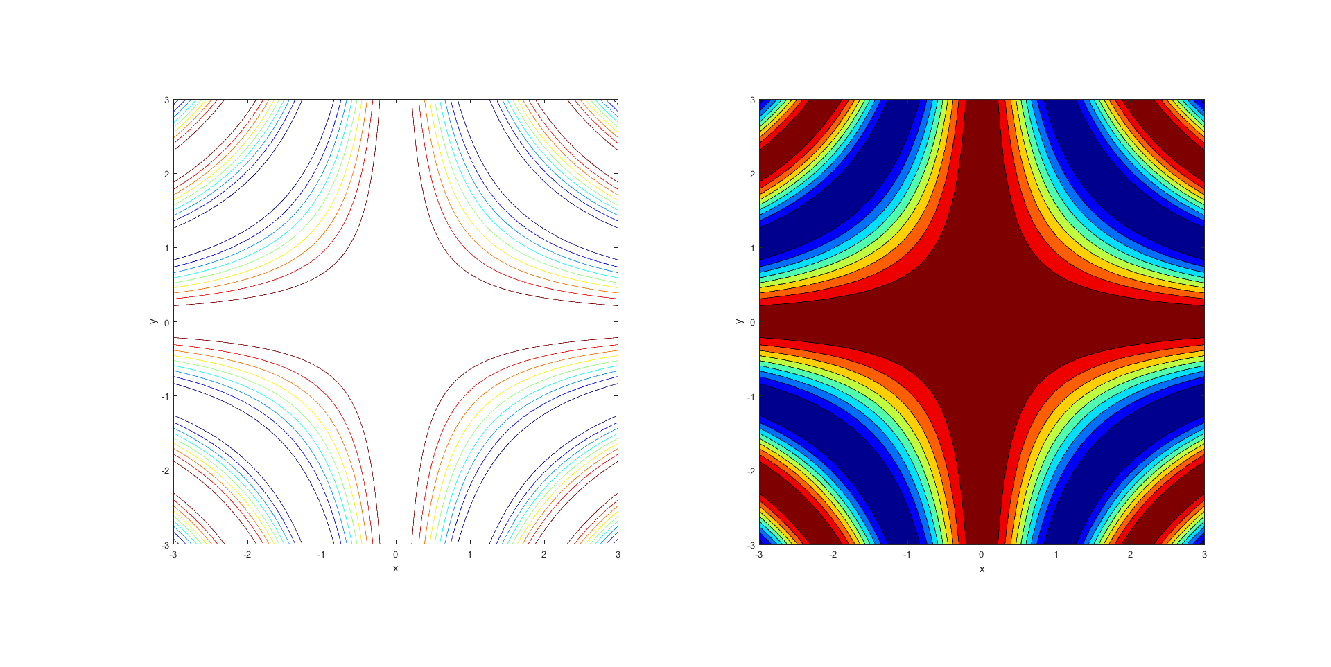
Normally you see the (closed) contour plots as 2-dimensional figures.

>> x = linspace(-3,3,500); 
>> y = linspace(-3,3,500); 
>> [x,y] = meshgrid(x,y); 
>> z = cos(x.*y); 
>> fig = figure('Color','White'); 
>> ax1 = subplot(1,2,1); 
>> colormap(jet) 
>> contour(x,y,z,'Parent',ax1); 
>> axis square 
>> xlabel('x') 
>> ylabel('y') 
>> ax2 = subplot(1,2,2); 
>> colormap(jet) 
>> contourf(x,y,z,'Parent',ax2); 
>> xlabel('x') 
>> ylabel('y') 
>> axis square