Exercise 1

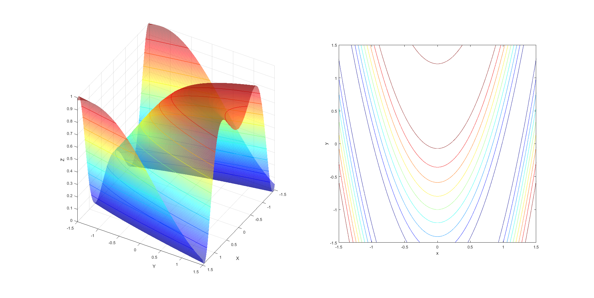
In order to plot the graph of the function $$f(x,y)=\tfrac{1}{2}\!\bigl(1-\sin(2x^2-y-1)\bigr)$$ we make a mesh grid and use the command surf to create surface plot. The command contour results in contours in 3D without a surface. We combine both commands for the desired result. To ensure that the contours are visible, we put the 'Face Alpha' property of the surface on $0.5$ to change opacity. We use subplot to show both the 3D surface plot and the regular 2D contour plot.

>> x = linspace(-3,3,500); 
>> y = linspace(-3,3,500); 
>> [x,y] = meshgrid(x,y); 
>> z = 0.5.*(1-sin(2.*x.^2-y-1)); 
>> fig = figure('Color','White'); 
>> ax1 = subplot(1,2,1); 
>> surf(x,y,z,'EdgeColor','none','FaceAlpha',0.5) 
>> colormap(jet) 
>> hold on 
>> contour3(x,y,z) 
>> xlabel('X') 
>> ylabel('Y') 
>> zlabel('Z') 
>> xlim([-1.5,1.5]) 
>> ylim([-1.5,1.5]) 
>> zlim([0,1]) 
>> view(120,35) 
>> ylim([-1.5,1.5]) 
>> ax2 = subplot(1,2,2); 
>> contour(x,y,z,'Parent',ax2); 
>> colormap(jet) >> xlabel('x') 
>> ylabel('y') >> xlim([-1.5,1.5]) 
>> ylim([-1.5,1.5]) 
>> axis square

This gives the following result:

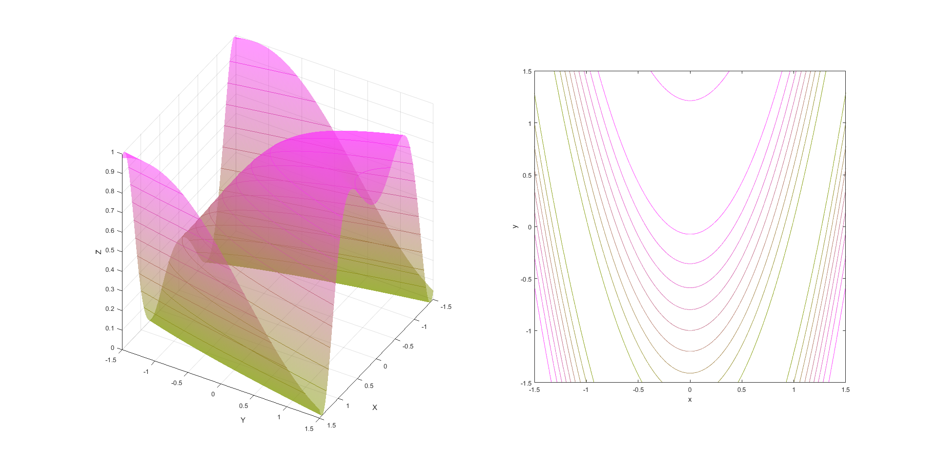
If you have made your own colormap, you could have done the following:

>> x = linspace(-3,3,500); 
>> y = linspace(-3,3,500); 
>> [x,y] = meshgrid(x,y); 
>> z = 0.5.*(1-sin(2.*x.^2-y-1));
>> fig = figure('Color','White'); 
>> ax1 = subplot(1,2,1); 
>> surf(x,y,z,'EdgeColor','none','FaceAlpha',0.5) 
>> % Definition of a 256x3 matrix with R,G and B values 
>> C = [linspace(0.5,1,256)', linspace(0.6,0.2,256)', linspace(0,1,256)']; 
>> colormap(C) 
>> hold on 
>> contour3(x,y,z) 
>> xlabel('X') 
>> ylabel('Y') 
>> zlabel('Z') 
>> xlim([-1.5,1.5]) 
>> ylim([-1.5,1.5]) 
>> zlim([0,1]) 
>> view(120,35) 
>> ylim([-1.5,1.5]) 
>> ax2 = subplot(1,2,2); 
>> contour(x,y,z,'Parent',ax2); 
>> colormap(C) 
>> xlabel('x') 
>> ylabel('y') 
>> xlim([-1.5,1.5]) 
>> ylim([-1.5,1.5]) 
>> axis square

This gives the following result:

Exercise 2

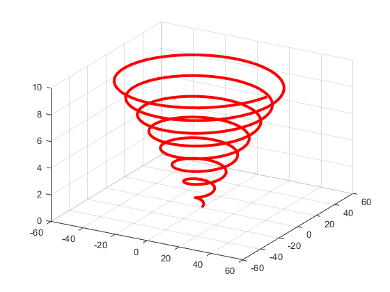
In order to plot the graph of the parametric curve $$f(t)=(t\cos t, t\sin t, \tfrac{1}{5}t)$$ on the interval $[0,50]$ we do the following:

>> t = linspace(0,50,500); 
>> xt = t.*cos(t); 
>> yt = t.*sin(t); 
>> zt = 0.2.*t; 
>> fig = figure('Color','White'); 
>> plot3(xt,yt,zt,'r','LineWidth',3) 
>> grid on 
>> xlim([-60,60]) 
>> ylim([-60,60]) 
>> zlim([0,10]) 
>> ax = gca; 
>> ax.XTick = [-60:20:60]; 
>> ax.YTick = [-60:20:60]; 
>> ax.ZTick = [0:2:10]; 
>> view(30,30)

The result is as follows: