Systems of differential equations: Linear systems of differential equations
 Drawing a phase portrait in MATLAB
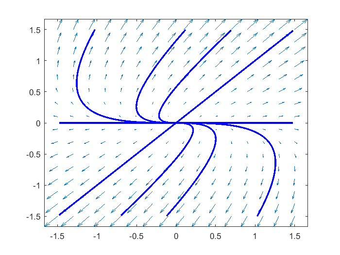
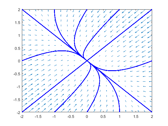
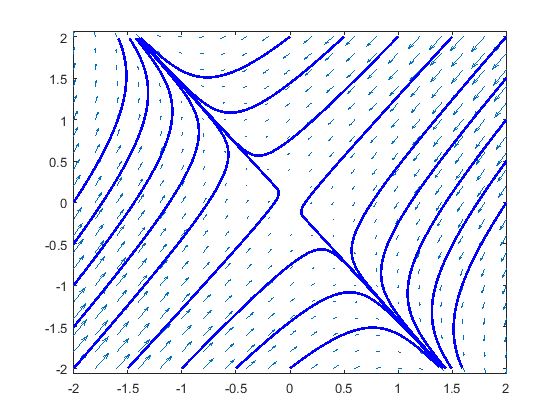
In the previous theory blocks , we have introduced the phase portrait of a linear system of two differential equations and we have plotted phase portratis for several real eigenvalues. Constructing a phase portrait by hand is a lot of work, but with mathematical software it is rather easily done. For example, in MATLAB you construct a vector field via the quiver function (with or scaled vectors) and with the the streamline command you can plot solution curves from given initial points. The following examples illustrate this.
Two positive eigenvalues \[\left\{\begin{aligned} \frac{\dd x}{\dd t} &= x+ 2 y\\[0.25cm] \frac{\dd y}{\dd t} &= 3y\end{aligned}\right.\]
>> [x,y] = meshgrid(-1.5:0.2:1.5, -1.5:0.2:1.5);
 >> dxdt = x + 2*y;
 >> dydt = 3*y;
 >> figure
 >> quiver(x, y, dxdt, dydt), axis tight % teken vectorveld
 >> % specificeer startpunten
 >> startx = [-0.2, -0.1, -0.05, -0.001, -0.001, 0.001, 0.001, 0.05, 0.1, 0.2];
 >> starty = [ 0.001, 0.001, 0.001, 0, -0.001, 0.001, 0, -0.001, -0.001, -0.001];
 >> set(groot,'defaultLineLineWidth',2) % verander default lijnbreedte
 >> streamline(x ,y, dxdt, dydt, startx, starty) % teken oplossingen
Two negative eigenvalues \[\left\{\begin{aligned} \frac{\dd x}{\dd t} &= -2x-y\\[0.25cm] \frac{\dd y}{\dd t} &= -x - 2y\end{aligned}\right.\]
>> [x,y] = meshgrid(-1.5:0.2:1.5, -1.5:0.2:1.5);
 >> dxdt = -2*x - y;
 >> dydt = -x - 2*y;
 >> figure
 >> quiver(x, y, dxdt, dydt), axis tight % teken vectorveld
 >> % specificeer startpunten
 >> startx = [-2, -1, 0, 1, 2, -2, -1, 0, 1, 2, -2, 2];
 >> starty = [-2, -2, -2, -2, -2, 2, 2, 2, 2, 2, 0, 0];
 >> set(groot,'defaultLineLineWidth',2) % verander default lijnbreedte
 >> streamline(x ,y, dxdt, dydt, startx, starty) % teken oplossingen
A positive and negative eigenvalues \[\left\{\begin{aligned} \frac{\dd x}{\dd t} &= -x-y\\[0.25cm] \frac{\dd y}{\dd t} &= -2x - y\end{aligned}\right.\]
>> [x,y] = meshgrid(-1.5:0.2:1.5, -1.5:0.2:1.5);
 >> dxdt = -x - y;
 >> dydt = -2*x - y;
 >> figure
 >> quiver(x, y, dxdt, dydt), axis tight % teken vectorveld
 >> % specificeer startpunten
 >> startx = [-2, -1.5, -1, -0.5, 0, -2, -2, -2, -2, 0, 0.5, 1, 1.5, 2, 2, 2, 2, 2];
 >> starty = [-2, -2, -2, -2, -2, -1.5, -1, -0.5, 0, 2, 2, 2, 2, 2, 1.5, 1. 0.5, 0];
 >> set(groot,'defaultLineLineWidth',2) % verander default lijnbreedte
 >> streamline(x ,y, dxdt, dydt, startx, starty) % teken oplossingen


