We consider the system of differential equations \[\left\{\begin{aligned} \dfrac{\dd x}{\dd t} &= -x+x^3\\[0.25cm] \dfrac{\dd y}{\dd t} &= -2y \end{aligned}\right.\] Equilibria exist when \(\dfrac{\dd x}{\dd t}=0\) and \(\dfrac{\dd y}{\dd t}=0\), so when\(-x+x^3=x(x-1)(x+1)=0\) and \(y=0\). Thus, there are three equilibria: \((0,0)\), \((1,0)\) and \((-1, 0)\).

We now find out what kind of equilibria we have for this system of differential equations. The general form of the Jacobian matrix in \((x,y)\) is \[J(x,y) =\matrix{\dfrac{\partial (-x+x^3)}{\partial x} & \dfrac{\partial (-x+x^3)}{\partial y}\\ \dfrac{\partial (-2y)}{\partial x} & \dfrac{\partial (-2y)}{\partial y}}=\matrix{-1+3x^2 & 0\\ 0 & -2}\]

• The corresponding linearisation in \((0,0)\) is \[\cv{ x'\\ y'}=\matrix{-1 & 0\\ 0 & -2}\cv{x\\ y}\] The eigenvalues of the Jacobian matrix are negative and thus all solutions near \((0,0)\) approach the origin. The origin is an attracting equilibrium.
• The corresponding linearisation in \((\pm 1,0)\) is \[\cv{ x'\\ y'}=\matrix{2 & 0\\ 0 & -2}\cv{x\\ y}\] The eigenvalues of the Jacobian matrix are positive and negative, and thus is \((\pm 1,0)\) a saddle point, in the sense that solution curves in one direction move toward the equilibrium, but in the other direction move away from it.

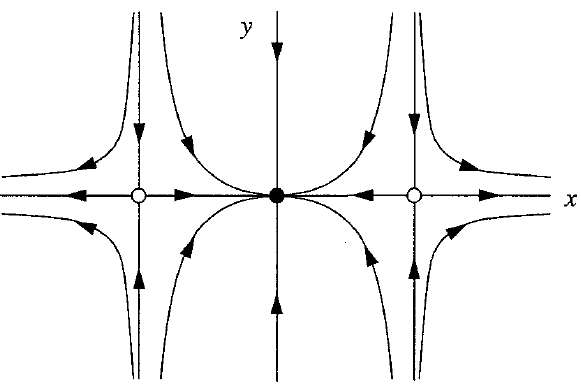
Because the differential equations are uncoupled, that is to say, two first-order ODEs that are separate from one another, we can easily check the analysis above: in the \(y\)-direction all solutions move toward \(y=0\); in the \(x\)-direction, the 1-dimensional phase portrait has an attracting equilibrium in \(x=0\) and two repelling equilibria in \(x=-1\) and \(x=1\). The two-dimensional phase portrait can be sketched as follows.

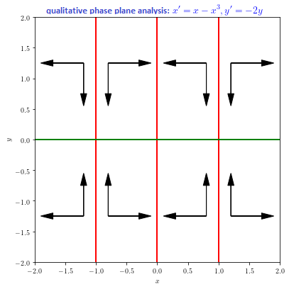
In qualitative sense, you can determine the following diagram of directions:

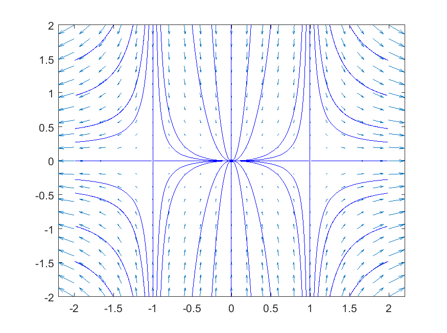
This corresponds with the phase portrait below, created in MATLAB.

>> [x,y] = meshgrid(-2:0.2:2, -2:0.2:2)
>> dxdt = -x+x.^3; 
>> dydt = -2*y; 
>> figure 
>> quiver(x, y, dxdt, dydt), axis tight % draw the vector field 
>> startx = [-1.5 -1.25 -1.1 -1.05 -1 -0.95 -0.9 -0.5 -0.25 0 0.25 0.5 0.9 0.95 1 1.05 1.1 1.25 1.5]; 
>> starty = -2*ones(size(startx)); 
>> streamline(x, y, dxdt, dydt, startx, starty) % draw solution curves
>> starty = 2*ones(size(startx)); 
>> streamline(x, y, dxdt, dydt, startx, starty) 
>> startx = [-1.01 -.99 0.99 1.01]; 
>> starty = [0 0 0 0]; 
>> streamline(x, y, dxdt, dydt, startx, starty)