Systems of differential equations: Linear systems of differential equations
 Drawing a phase portrait in R
The phaseR package provides facilities to draw a direction field for a system of differential equations and only solution curves drawing herein. The following examples illustrate this. It does not have to be a linear system of differential equations, but we restrict ourselves here to such examples.
Twee positieve eigenwaarden \[\left\{\begin{aligned} \frac{\dd x}{\dd t} &= x+ 2 y\\[0.25cm] \frac{\dd y}{\dd t} &= 3y\end{aligned}\right.\]
>> library(phaseR)
>> model <- function(tijd, begintoestand, parameters){
     with(as.list(c(begintoestand, parameters)),{
       dxdt <- x + 2*y
       dydt <- 3*y
       return(list(c(dxdt, dydt)))
     })
   }
>> flowField(model, xlim = c(-1.5, 1.5), ylim = c(-1.5, 1.5),
             system = "two.dim", state.names = c("x", "y"), points = 16,
             add = FALSE, xlab ="x", ylab ="y", col="turquoise")
>> initvals <- matrix(c(-0.2,-0.1,-0.05,-0.001,-0.001,0.001,0.001,0.05,0.1,0.2,
                        0.001,0.001,0.001,0,-0.001,0.001,0,-0.001,-0.001,-0.001),
                      nrow=10, ncol=2, byrow=FALSE)
>> trajectory(model, y0 = initvals, tlim = c(0, 25),
              state.names = c("x", "y"), lwd = 2, col="blue", cex = 0.1)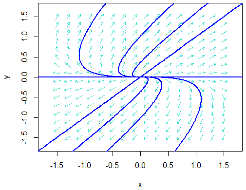
Twee negatieve eigenwaarden \[\left\{\begin{aligned} \frac{\dd x}{\dd t} &= -2x-y\\[0.25cm] \frac{\dd y}{\dd t} &= -x - 2y\end{aligned}\right.\]
>> library(phaseR)
>> model <- function(tijd, begintoestand, parameters){
     with(as.list(c(begintoestand, parameters)),{
       dxdt <- -2*x - y
       dydt <- -x - 2*y
       return(list(c(dxdt, dydt)))
     })
   }
>> flowField(model, xlim = c(-1.5, 1.5), ylim = c(-1.5, 1.5),
             system = "two.dim", state.names = c("x", "y"), points = 16,
             add = FALSE, xlab ="x", ylab ="y", col="turquoise")
>> initvals <- matrix(c(-2, -1,  0,  1,  2, -2, -1, 0, 1, 2, -2, 2,
                      -2, -2, -2, -2, -2,  2,  2, 2, 2, 2,  0, 0),
                    nrow=12, ncol=2, byrow=FALSE)
>> trajectory(model, y0 = initvals, tlim = c(0, 25),
              state.names = c("x", "y"), lwd = 2, col="blue", cex = 0.1)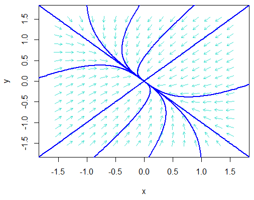
Two negative eigenvalues \[\left\{\begin{aligned} \frac{\dd x}{\dd t} &= -2x-y\\[0.25cm] \frac{\dd y}{\dd t} &= -x - 2y\end{aligned}\right.\]
>> library(phaseR)
>> model <- function(tijd, begintoestand, parameters){
     with(as.list(c(begintoestand, parameters)),{
       dxdt <- -2*x - y
       dydt <- -x - 2*y
       return(list(c(dxdt, dydt)))
     })
   }
>> flowField(model, xlim = c(-1.5, 1.5), ylim = c(-1.5, 1.5),
             system = "two.dim", state.names = c("x", "y"), points = 16,
             add = FALSE, xlab ="x", ylab ="y", col="turquoise")
>> initvals <- matrix(c(-2, -1,  0,  1,  2, -2, -1, 0, 1, 2, -2, 2,
                      -2, -2, -2, -2, -2,  2,  2, 2, 2, 2,  0, 0),
                    nrow=12, ncol=2, byrow=FALSE)
>> trajectory(model, y0 = initvals, tlim = c(0, 25),
              state.names = c("x", "y"), lwd = 2, col="blue", cex = 0.1)

A positive and a negative eigenvalues \[\left\{\begin{aligned} \frac{\dd x}{\dd t} &= -x-y\\[0.25cm] \frac{\dd y}{\dd t} &= -2x - y\end{aligned}\right.\]
>> library(phaseR)
>> model <- function(tijd, begintoestand, parameters){
     with(as.list(c(begintoestand, parameters)),{
       dxdt <- -x - y
       dydt <- -2*x - yy
       return(list(c(dxdt, dydt)))
     })
   }
>> flowField(model, xlim = c(-2, 2), ylim = c(-2, 2),
             system = "two.dim", state.names = c("x", "y"), points = 21,
             add = FALSE, xlab ="x", ylab ="y", col="turquoise")
>> initvals <- matrix(c(-2,-1.5,-1,-0.5,0,-2,-2,-2,-2,0,0.5,1,1.5,2,2,2,2,2,
                        -2,-2,-2,-2,-2,-1.5,-1,-0.5,0,2,2,2,2,2,1.5,1,0.5,0),
                      nrow=18, ncol=2, byrow=FALSE)
>> trajectory(model, y0 = initvals, tlim = c(0, 25),
              state.names = c("x", "y"), lwd = 2, col="blue", cex = 0.1)