Multiple integrals: Double integrals
 Double integrals approximated with a Riemann sum
How do you calculate a double integral numerically? We are going to approach this in the same way as numerically integrating functions of one variable. We do it again only for a positive continuous function \(f(x,y)\) defined on a rectangle \(R=[a,b]\times [c,d]\).
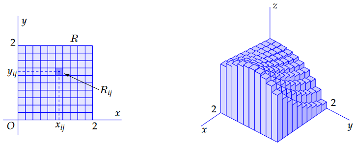
Approach with Riemann sums We always divide the interval \([a,b]\) on the \(x\)-axis into \(m\) pieces by designating fixed points \(x_0, x_1, x_2,\ldots, x_m\) with \[a = x_0 < x_1 < x_2 < \cdots < x_m = b\] in that interval. Similarly, we divide the interval \([c,d]\) on the \(y\)-axis into \(n\) pieces by designating fixed points \(y_0, y_1, y_2,\ldots, y_n\) with \[c = y_0 < y_1 < y_2 < \cdots < y_n = d\] in that interval. This way we get \(m\times n\) sub-rectangles \(R_{ij}= [x_{i-1},x_i]\times [y_{i-1},y_i]\) with \(i=1,2,\ldots m\) and \(j=1,2,\ldots m\). Such a set is called a partition \(\mathcal{V}\) of \([a,b]\times [c,d]\). We then choose a random point \(s_{ij}\) in each of the sub-rectangles \(R_{ij}\); we call such point a tag. So \(x_{i-1}\le s_{ij}\le x_i\) for \(i = 1, 2, \ldots m\) and \(y_{j-1}\le s_{ij}\le y_j\) for \(j = 1, 2, \ldots n\). We denote the area of each sub-rectangle \(R_{ij}\) with \({\vartriangle}_{ij}={\vartriangle}_{i}\cdot {\vartriangle}_{j}\), where \({\vartriangle}_{i}=x_i-x_{i-1})\) and \({\vartriangle}_{j}=x_j-x_{j-1})\) are the width and height of each sub-rectangle \(R_{ij}\). We call the maximum of the lengths of the sides of the partial rectangles the mesh size. The expression \[S(\mathcal{V}; s_{11}, \ldots, s_{mn})=\sum_{i=1}^m\sum_{j=1}^{n}f(s_{ij})\cdot {\vartriangle}_{ij}\] is called a Riemann sum corresponding with the function \(f\). Note: for a given partition \(\mathcal{V}\) of \([a, b]\times [c,d]\) there are many different Riemann sums: with each choice of tags you always get one. Such a Riemann sum is therefore the sum of the volume of rectangular pillars with the sub-rectangles used in the partition as bases. The volume of these rectangular pillars (i.e, cuboids) add up to an approximation of the volume under a graph that we want to calculate. The requested volume is, in a sense, a limit of such Riemann sums. See example below.

In the figure above, for the function \(f(x,y)=\frac{1}{6}(x^2y+2\sqrt{x+1}-y^3+6)\), we have the square \([0,2]\times[0,2]\) as integration region \(R\), an evenly divided partition of \(R\) with \(10^2=100\) sub-squares \(m=n=10\), \(\vartriangle_{i}=\vartriangle_{j}=0.2\) for all \(i,j=1,2,\ldots 10\) (the mesh size is equal to \(0.2\)), and in each sub-square \(R_{ij}\) we have choen the centre point for \(s_{ij}\). Then, in eight significant figures, we get the Riemann sum \[\sum_{i=1}^{10}\sum_{j-1}^{10}f(s_{ij})\cdot {\vartriangle}_{ij} \approx 5.4251910\] The smaller the mesh size of the partition, the better the approximation. For example, if you divide the square evenly into \(10^4=1000\) sub-squares and the mesh size is therefore equal to \(0.02\), you get \[\sum_{i=1}^{100}\sum_{j-1}^{100}f(s_{ij})\cdot {\vartriangle}_{ij} \approx 5.4205590\] If you do the same with a mesh size of \(0.002\), you get \[\sum_{i=1}^{1000}\sum_{j-1}^{1000}f(s_{ij})\cdot {\vartriangle}_{ij} \approx 5.4205127\] and the first six decimal places are already good compared to the exact result \(\frac{29}9+4/3\sqrt{3}\approx 5.420512188\) for the double integral: \[\begin{aligned}\iint_R f(x,y)\,\dd(x,y) &= \lim_{n\to\infty}\left(\lim_{m\to\infty}f(s_{ij})\cdot {\vartriangle}_{i}\right)\cdot {\vartriangle}_{j}=\int_{y=0}^{y=2}\left(\int_{x=0}^{x=2}f(x,y)\,\dd x\right)\dd y\\[0.25cm] &= \lim_{m\to\infty}\left(\lim_{n\to\infty}f(s_{ij})\cdot {\vartriangle}_{j}\right)\cdot {\vartriangle}_{i}=\int_{x=0}^{x=2}\left(\int_{y=0}^{y=2}f(x,y)\,\dd y\right)\dd x\end{aligned}\]
Step-by-step approach for a numerical calculation of a double integral Even though there are much better methods to calculate a double integral numerically, the Riemann integration method described above does give a good idea of what a double integral actually is. We can draw up a step-by-step approach that can be applied more broadly:
- Divide the integration region \(R\) into small sub-regions \(\dd R\), which are also called area elements.
- Choose the area elements so small that the function above them is almost constant.
- Choose any point \((x,y)\) in each area element \(\dd R\) and calculate \(f(x,y)\). Multiply this by the area \(|\dd R|\) of \(\dd R\).
- Add up all the results obtained in step 3. The sum is then approximately equal to the double integral. The approximation is better when the area elements are smaller.


