Double integrals as iterated integrals

Multiple integrals: Double integrals

Double integrals as iterated integrals

In the previous theory pages it has already been suggested that a double integral can also be calculated exactly by repeated integration. We will get into this in a bit more detail.

Suppose that we want to calculate a double integral $\iint_R f(x,y)\,\dd(x,y)$ for a positive continuous function $f$ over a rectangular region of integration $R=[a,b]\times [c,d]$ . Define the following auxiliary function $S(y)=\int_{x=a}^{x=b} f(x,y)\,\dd x$ With a fixed $y$ you therefore integrate the function $f(x,y)$ to $x$ .

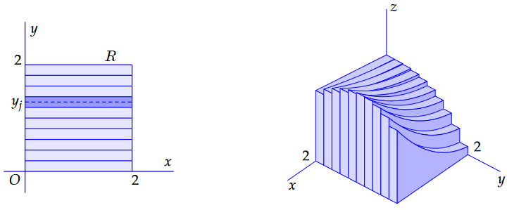
Divide the region $R$ into $m$ strips of length ${\vartriangle}y=(d-c)/m$ . In each strip, choose a horizontal line at height $y_j$ and calculate $S(y_j)$ . This gives the area under the graph of $f(x,y_j)$ and then the product of this with ${\vartriangle}y$ is equal to the volume of the `slice' with thickness ${\vartriangle}y$ that has the graph of the function $f(x,y_j)$ as profile ( $x$ is the variable here, $y_j$ is fixed).

In the figure below we have again chosen the function $f(x,y)=\frac{1}{6}(x^2y+2\sqrt{x+1}-y^3+6)$ and the square $[0,2]\times[0,2]$ as region of integration $R$ . $10$ horizontal strips have been taken ( $m=10,{\vartriangle}y=0.2$ ). The 'slices' of which each height always fits the centre of the relevant strip can be seen on the right. herhaalde integratie: eerst naar y, dan naar x

The area of that profile is $S(y_j)$ and the sum $\sum_{j=1}^{m}S(y_j)\cdot {\vartriangle}y$ is again an approximation of the double integral $\iint_R f(x,y)\,\dd(x,y)$ . At the same time it is also an approximation of the integral $\int_{y=c}^{y=d} S(y)\,\dd y$ . For 'neat' functions, both integrals are equal: $\iint_R f(x,y)\,\dd(x,y)=\int_{y=c}^{y=d} S(y)\,\dd y= \int_{y=c}^{y=d}\left(\int_{x=a}^{x=b} f(x,y)\,\dd x\right)\dd y$

In the example of the function $f(x,y)=\frac{1}{6}(x^2y+2\sqrt{x+1}-y^3+6)$ and the square $[0,2]\times[0,2]$ as region of integration $R$ we get $\begin{aligned} S(y) &= \int_{x=0}^{x=2} f(x,y)\,\dd x\\[0.25cm] &= \int_{x=0}^{x=2}\frac{1}{6}(x^2y+2\sqrt{x+1}-y^3+6)\,\dd x \\[0.25cm] &=\Bigl[\frac{1}{18}x^3y+\frac{2}{9}(x+1)^{\frac{3}{2}}-\frac{1}{6}xy^3+x\Bigr]_0^{2}\\[0.25cm] &= \bigl(\frac{4}{9}y+\frac{2}{9}\sqrt{27}-\frac{1}{3}y^3+2\bigr)-\frac{2}{9}\\[0.25cm] &= \frac{4}{9}y+\frac{2}{3}\sqrt{3}-\frac{1}{3}y^3+\frac{16}{9}\end{aligned}$ and therefore $\begin{aligned}\iint_R f(x,y)\,\dd(x,y) &= \int_{y=0}^{y=2} S(y)\,\dd y\\[0.25cm] &= \int_{y=0}^{y=2}\left(\frac{4}{9}y+\frac{2}{3}\sqrt{3}-\frac{1}{3}y^3+\frac{16}{9}\right)\dd y\\[0.25cm] &= \Bigl[\frac{2}{9}y^2+\frac{2}{3}\sqrt{3}y-\frac{1}{12}y^4+\frac{16}{9}y\Bigl]_{0}^{2}\\[0.25cm] &=\frac{8}{9} + \frac{4}{3}\sqrt{3}-\frac{16}{12}+\frac{32}{9}\\[0.25cm] &= \frac{28}{9}+\frac{4}{3}\sqrt{3}\end{aligned}$

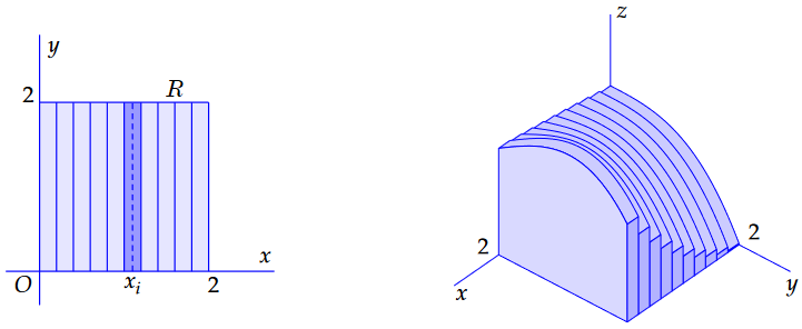
Above we first integrated to $x$ and then to $y$ . But the order can also be reversed. The double integral then becomes $\iint_R f(x,y)\,\dd(y,x)= \int_{x=a}^{x=b}\left(\int_{y=c}^{y=d} f(x,y)\,\dd y\right)\dd x$ The result of iterated integration is the same, but the route is different. In the derivation of this formula you now start with the introduction of the auxiliary function $T(x)=\int_{y=c}^{y=d} f(x,y)\,\dd y$ With a fixed $x$ you integrate the function $f(x,y)$ to $y$ . After this you divide the region $R$ into $n$ vertical strips of length ${\vartriangle}x=(b-a)/n$ . In each strip, choose a vertical line of width $x_i$ and calculate $T(x_i)$ . This gives the area under the graph of $f(x_i,y)$ and the product of this with ${\vartriangle}x$ is then equal to the volume of the `slice' with thickness ${\vartriangle}x$ that has the graph of the function $f(x_i,y)$ as profile ( $y$ is the variable here, $x_i$ is fixed). Below is the strip partition and the slices approximation of the double integral for the above example.

herhaalde integratie: eerst naar x, dan naar y

The area of the profile $f(x_i,y)$ is $T(x_i)$ and the sum $\sum_{j=1}^{x=b}T(x_j)\cdot {\vartriangle}x$ is again an approximation of the double integral $\iint_R f(x,y)\,\dd(y,x)$ . At the same time it is also an approximation of the integral $\int_{x=a}^{x=b} T(x)\,\dd x$ . For 'neat' functions, both integrals are equal to each other: $\iint_R f(x,y)\,\dd(y,x)=\int_{x=a}^{x=b} T(x)\,\dd x= \int_{x=a}^{x=b}\left(\int_{y=c}^{y=d} f(x,y)\,\dd y\right)\dd x$ To avoid using parentheses, the notation $\dd(y,x)=\dd y\,\dd x$ is interpreted as repeated integration with first integrating to $y$ and then integrating to $x$ . The notation $\dd(x,y)=\dd x\,\dd y$ is the other way around: first integrate to $x$ and only then integrate to $y$ . With 'neat' functions this produces the same result. Sometimes you have to make a well-considered choice of integration order because of the simplicity of the calculation.

Calculate $\iint_R (9+x-2y)\,\dd(x,y)$ with $R=[0,2]\times [2,4]$

$\displaystyle \iint_R (9+x-2y)\,\dd(x,y)={}$ $16$

$\begin{aligned} \iint_R (9+x-2y)\,\dd(x,y) &= \int_{y=2}^{y=4}\left(\int_{x=0}^{x=2}(9+x-2y)\,\dd x\right)\dd y\\[0.25cm] &=\int_{y=2}^{y=4}\biggl[9x+{{1}\over{2}}x^2-2xy\biggr]_{x=0}^{x=2}\,\,\dd y\\[0.25cm] &= \int_{y=2}^{y=4}\left(20-4\,y\right)\dd y\\[0.25cm] &=\biggl[20\,y-2\,y^2\biggr]_{y=2}^{y=4}\\[0.25cm] &= 48-32\\[0.25cm] &=16\end{aligned}$

You get the same result according to Fubini's theorem by reversing the integration variables: $\begin{aligned} \iint_R (9+x-2y)\,\dd(x,y) &= \int_{x=0}^{x=2}\left(\int_{y=2}^{y=4}(9+x-2y)\,\dd y\right)\dd x\\[0.25cm] &=\int_{x=0}^{x=2}\biggl[9y+xy-y^2\biggr]_{y=2}^{y=4}\,\,\dd x\\[0.25cm] &= \int_{x=0}^{x=2}\biggl(\bigl(4\,x+20\bigr)-\bigl(2\,x+14\bigr)\biggr)\,\dd x\\[0.25cm] &= \int_{x=0}^{x=2}\left(2\,x+6\right)\dd x\\[0.25cm] &=\biggl[x^2+6\,x\biggr]_{x=0}^{x=2}\\[0.25cm] &= 2^2+6\times 2\\[0.25cm] &=16\end{aligned}$

New example