Arbitrary periodic signals

Trigonometry: Trigonometric functions

Arbitrary periodic signals

An arbitrary signal $s(t)$ is periodic with period $T$ (also known as vibration time) when $T$ is the smallest positive number with the property that

$s(t+T)=s(t)$ for all $t$ .

For such a signal, the frequency $f$ is again defined as

$f=\frac{1}{T}$ The number $f$ is the number of periods ("vibrations") per unit of time.
As a rule, $f$ is the number of vibrations per second; one measures the frequency in hertz (Hz).

The equilibrium value of such a signal is understood ad the mean value over one period.
The amplitude of $s(t)$ is the maximum deviation from the equilibrium value.

The graph of the signal

$s(t)=1+2\sin(2\pi t)+\sin(4\pi t)$ is shown below, together with the equilibrium value which is equal to 1.
The amplitude can be calculated exactly: the function takes on the displayed time interval the maximum value for $t=\tfrac{1}{6}$ and this value is equal to $1+\tfrac{3}{2}\!\sqrt{3}$ . The amplitude of the signal is thus equal to $\tfrac{3}{2}\!\sqrt{3}\approx 2.6$ .

graph of a periodic signal

The above example may seem artifical, but you come across many periodic signals in practice. We give two examples, one from biomechanics and the other from tidal analysis.

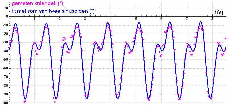
This example comes from biomechanics and is about the knee angle (in degrees) during hopping.
Measurements on video images of the movement are plotted in the below figure along with the graph of an approximation with two sinusoids and a constant. The mathematical formula of this approach is

$\mathrm{knee\;angle\;}({}^{\circ})=-45.0+31.0\cdot\sin(2\pi\cdot 0.82\cdot t+1.11)+21.1\cdot\sin(2\pi\cdot1.65\cdot t-1.74)$ The frequency of the signal is therefore approximately equal to $0.82$ Hz. The equilibrium value is approximately equal to $-45^{\circ}$ and the amplitude is equal to $50^{\circ}$ . These two values cannot be read from the graph, but must be determined numerically over a period.

graph of a knee angle

This is an example of tidal analysis. We have chosen here for the analysis of the tide in Sewells Point (Virginia, USA) on March 23-25 March 2006. Measured data are plotted in the below figurealong with the graph of an approximation with three sinusoids and a constant. The mathematical formula for this approach is

$\begin{eqnarray*}\mathrm{water\;level\;(cm)} &=& 40.9+31.0\cdot\sin(0.506\cdot t-2.463) \\ & & +8.8\cdot\sin(0.535\cdot t+0.165)+7.7\sin(0.251\cdot t=0.745)\end{eqnarray*}$

graph of a tide