Limited exponential growth: Applications of limited exponential growth models
 Reaction kinetics of a unimolecular equilibrium reaction
forward \(\displaystyle \text{A}\stackrel{k_1}{\longrightarrow} \text{B}\) with reaction rate constant \(k_1\)
backward \(\displaystyle \text{B}\stackrel{k_{2}}{\longrightarrow} \text{A}\) with rate constant \(k_{2}\)
Species A is not only converted into B, but it is also formed from species B by the reverse reaction. Similarly substance B is not only formed, but disappears again by the reverse reaction. When we assume elementary chemical reactions in this system, then the following two coupled differential equations describe the reaction kinetics: \[\left\{\begin{aligned}\frac{\dd[\text{A}]}{\dd t}&=-k_1[\text{A}]+k_{2}[\text{B}]\\ \\ \frac{\dd[\text{B}]}{\dd t}&=k_1[\text{A}]-k_{2} [\text{B}]\end{aligned}\right.\] Under the assumption that the total concentration of A and B is constant, we can uncouple the differential equations: if \([\text{A}]+[\text{B}]=K\) for some constant \(K\), then you can rewrite the equations as \[\begin{aligned}\frac{\dd[\text{A}]}{\dd t}&=-k_1 [\text{A}]+k_{2} (K-[\text{A}])\\ \\ \frac{\dd[\text{B}]}{\dd t}&=k_1 (K-[\text{B}])-k_{2}[\text{B}]\end{aligned}\] So: \[\begin{aligned}\frac{\dd[\text{A}]}{\dd t}&=k_{2} K-(k_1+k_{2}) [\text{A}]\\ \\ \frac{\dd[\text{B}]}{\dd t}&=k_1 K-(k_1+k_{2}) [\text{B}]\end{aligned}\] Both equations correspond with restricted exponential growth, and an equilibrium settles in after sufficient time.
There is chemical equilibrium when \[\frac{\dd[\text{A}]}{\dd t}=0, \frac{\dd[\text{B}]}{\dd t}=0\] The equilibrium concentrations \([\text{A}]_{\infty}\) and \([\text{B}]_{\infty}\) can be determined herewith; verify that the follwoing is true when the system is in equilibrium: \[[\text{A}]_{\infty}=\frac{k_{-1}\cdot c}{(k_1+k_{-1})},\quad [\text{B}]_{\infty}=\frac{k_{1}\cdot c}{(k_1+k_{-1})}\] In equilibrium, the concentrations are related as quotient of the forward and reverse reaction rate constants: \[\frac{[\text{A}]_{\infty}}{[\text{B}]_{\infty}} = \frac{k_{-1}}{k_{1}}\]
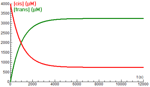
As a concrete example of an equilibrium reaction, consider the reaction kinetics of the isomerization
\[\mathit{cis\mbox{-}}\mathrm{Mo(CO)}_4 \mathrm{[P(}\mathit{n}\,\mbox{-}\mathrm{Bu)}_3\mathrm{]}_2\rightleftharpoons \mathit{trans\mbox{-}}\mathrm{Mo(CO)}_4 \mathrm{[P(}\mathit{n}\,\mbox{-}\mathrm{Bu)}_3\mathrm{]}_2\] The reaction rate constants (in \(\mathrm{s}^{-1}\) ) are dependent on the temperature \(T\) (in Kelvin) according to the following formulas (Bengali and Mooney, 2003): \[k_1=T\cdot 10^{8.87-\frac{5195}{T}},\quad k_{-1}=T\cdot 10^{8.78-\frac{5394}{T}}\] The diagram below shows the time profile of the concentrations of the cis- and trans-form (in uM) at a temperature of \(85{}^{\circ}\!\mathrm{C}\). Both curves are rooted in modelling of limited exponential growth.
Below are drawn the concentration-time curves at a temperature of \(80{}^{\circ}\!\mathrm{C}\). The previous curves for \(85{}^{\circ}\!\mathrm{C}\) are in gray.
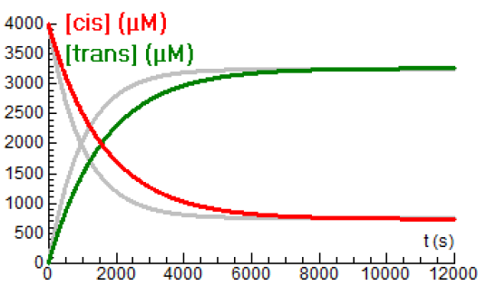
You see in the diagram that the equilibrium concentrations hartly diffe, but that one equilibrium is reached slower than the other equilibrium. Apparently, the ratio of the rate constants remains almost the same.
Bengali, AA & Mooney, KE (2003). Synthesis, kinetics, and thermodynamics: an advanced laboratory investigation of the cis-trans isomerization of \(\mathrm{Mo(CO)}_4\mathrm{(PR}_3\mathrm{)}_2.\) Journal of Chemical Education 80 (9), 1044-1047.


