The differential equation of limited exponential growth

Limited exponential growth: Limited exponential growth functions

The differential equation of limited exponential growth

In the introduction we have already seen the differential equation of limited exponential growth and we have solved the differential equation in two different contexts.

The general solution of the differential equation \[\frac{dy}{dt}=r\cdot(a-y)\] with constants \(a>0,\;r>0\) is \[y(t)=a-c\cdot e^{-r\cdot t}\] for some constant \(c\).

For the math enthusiast, we prove that the general solution of the differential equation \[\frac{dy}{dt}=r\cdot(a-y)\] with constants \(a>0,\;r>0\) is equal to \[y(t)=a-c\cdot e^{-r\cdot t}\] for some constant \(C\).

Start with a new quantity \(z(t)\) defines as \[z=y-a\] Then: \[\begin{aligned}\frac{dz}{dt}&=\frac{d(y-a)}{dt}\\ \\ &=\frac{dy}{dt}\\ \\ &= r\cdot(a-y)\\ \\ &= -r\cdot z\end{aligned}\] The quantity \(z\) therefore satisfies the differential equation of exponential decay, \(z'(t)=-r\cdot z(t)\), and the general solution can be written as \[z(t)=-c\cdot e^{-r\cdot t}\] for some constant \(c\). But then we know that \[y(t)=a+z(t)=a-c \cdot e^{-r\cdot t}\tiny.\]

Actually, you can solve the differential equation in another way (based on what is called an integrating factor). From \[\frac{dy}{dt}=r\cdot(a-y)\] follows \[\frac{\displaystyle\frac{dy}{dt}}{a-y}=r\] Now you may think that nothing is gained, but the left-hand side is the derivative of a known expression; with the chain rule you can rewrite \[\frac{d(-\ln\bigl(|a-y|\bigr)}{dt}=r\] in other words the derivative of \(\ln\bigl(|a-y|\bigr)\) must be equal to \(-r\). But then the functions \(\ln\bigl(|a-y|\bigr)\) and \(-r\cdot t\) differ only a constant, say \(C\) : \[\ln\bigl(|a-y|\bigr)=-r\cdot t + C\] or \[|a-y| = e^{-r\cdot t+C\] Then: \[y=a-c \cdot e^{-r\cdot t}\] with \(c=\pm e^C\).

Solve the following initial value problem: \[\frac{dy}{dt}=0.10\cdot(20-y),\quad y(1)=13\]

The differential equation models limited exponential growth and its general solution is \[y(t)=20-c\cdot e^{-0.10t}\] Because \(y(1)=13\) we can deduce the following equation for \(c\): \[13=20-c\cdot e^{-0.10\cdot 1}\] Thus: \[c\cdot e^{-0.1}=20-13=7\] Then: \[c=7\cdot e^{0.1}\approx 7.74\] The solution of the initial value problem is therefore
\[\begin{aligned} y(t)&=20-7\cdot e^{0.1}\cdot e^{-0.10t}\\ &\approx 20-7.74\cdot e^{-0.10t}\end{aligned}\]

New example

Asymptotics and stability Although we can solve this differential equation in explicit form, yet it is interesting to look at how the differential equation itself to get a lot of information about the possible solutions is.

For example, to know whether equilibria solutions exist and what they are, you can solve the equation\(\frac{dy}{dt}=0\) because the variable \(y\) does not change when the derivative is equal to 0. We speak of an equilibrium. In this case \(y(t)=a\) is the only equilibrium solution. If the quantity \(y\) at a certain time assumes a value smaller than \(a\), then the derivative is greater than zero and the solution curve increases at that moment. If the quantity \(y\) at a certain time assumes a value greater than \(a\), then the derivative is less than zero, and the solution curve decreases at that moment. So at small deviations from the equilibrium the solution gradually returns to equilibrium. We say that the equilibrium is attracting.

Behaviour of solutions displayed in a slope field To know how solutions of the differential equation behave near the equilibrium solution, you can also study the slope field. As a concrete example below is the slope field of the differential equation \[\frac{dy}{dt}=3-2y\] drawn together with two solution curves. The curves are constructed by following the line segments of the slope field in small time increments. In this case we have an attractive equilibrium: any solution curve near the equilibrium approaches the equilibrium. In this example an even stronger result holds: any solution approaches in the long run the equilibrium solution. Without knowing the solution explicitly, it is already possible to predict from the slope field how solutions will behave.

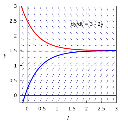
graphs of the limited exponential growth function

Interactive version of the slope field For those who want to understand the model better through the slope field: You can play with the interactive version of the slope field of a differential equation. As an example, the above differential equation of limited exponential growth is the default example and one of many possible solution curves is already drawn. But you can adjust the mathematical formula. By dragging point \(P\) you explore can different solution curves. You can change settings and then get a picture of the new situation with the update button.