Definition and basic properties

Logistic growth: The logistic function

Definition and basic properties

The logistic function, also called sigmoid function, is \[y(t)=\frac{a}{1+c\cdot e^{-r\cdot t}}\] with \(a>0\) and \(c>0\). The graph of this function in the case \(r>0\) is outlined below: the graph is an increasing sigmoid, i.e., an S-shaped curve: the growth is first increasing, and then progressively decreases and disappears over time so that the limit \(a\) will be approached. It holds that \(y(0)=\frac{a}{1+c}\) and \(y(t)\) approaches \(a\) with increasing time \(t\). The parameter \(a\) is called the carying capacity in the logistic growth model and \(r\) the intrinsic growth factor.

graph of logistic growth function

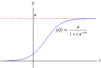
Consider how the graph \(y(t)\) looks like in case\(r<0\).

A special case of the logistic function is \[\sigma(x)=\frac{1}{1+e^{-x}}\] This function displays real values in between 0 and 1 and is widely used in neural network theory in order to limit response values.

The derivative of the logistic function \(\displaystyle y(t)=\frac{a}{1+c\cdot e^{-r\cdot t}}\) can be computed with the rules of differentiating and satisfies the relationship \[\frac{dy}{dt}=\frac{r}{a}\cdot y\cdot (a-y)\] This is the differential equation of logistic growth.
Sometimes it is written as \[\frac{dy}{dt}=r\cdot y\cdot \bigl(1-\frac{y}{a}\bigr)\] We speak of the logistic growth model, also known as the Verhulst model.

For the math enthusiast, we prove that the derivative of the logistic function \(\displaystyle y(t)=\frac{a}{1+c\cdot e^{-r\cdot t}}\) satisfies the relationship \[\frac{dy}{dt}=\frac{r}{a}\cdot y\cdot (a-y)\]

Uding the rules of differentiation we can determine the derivative \(y'(t)\): \[\begin{aligned}y(t)&=\frac{a}{1+c\cdot e^{-r\cdot t}}\\ \\ &=a\cdot\left(1+c\cdot e^{-r\cdot t}\right)^{-1}\end{aligned}\] The derivative is \[\begin{aligned}y'(t)&=-a\cdot\left(1+c\cdot e^{-r\cdot t}\right)^{-2}\cdot \left(c\cdot r\cdot e^{-r\cdot t}\right)\\ \\ &=\frac{a}{1+c\cdot e^{-r\cdot t}}\cdot \frac{c\cdot r\cdot e^{-r\cdot t}}{1+c\cdot e^{-r\cdot t}}\\ \\ &= \frac{a}{1+c\cdot e^{-r\cdot t}}\cdot \frac{r}{a}\cdot \frac{a\cdot c\cdot e^{-r\cdot t}}{1+c\cdot e^{-r\cdot t}}\end{aligned}\] because \[\begin{aligned}a-y(t)&=a-\frac{a}{1+c\cdot e^{-r\cdot t}}\\ \\ &=\frac{a\cdot c\cdot e^{-r\cdot t}}{1+c\cdot e^{-r\cdot t}}\end{aligned}\] therefore applies \[y'(t)=\frac{r}{a}\cdot y(t)\cdot \bigl(a-y(t)\bigr)\]

The general solution of the differential equation \[\frac{dy}{dt}=r\cdot y\cdot \bigl(1-\frac{y}{a}\bigr)\] with constants \(a>0\) and \(r\) is equal to \[y(t)=\frac{a}{1+c\cdot e^{-r\cdot t}}\] for some constant \(c\).

The constant \(c\) is often determined by the initial value \(y(0)\). Only in the case of \(c>0\), i.e., when \(y(0)\) is between 0 and \(a\), there is a logistic function with a sigmoid as function graph.

For math enthusiasts we give a proof. The clever trick consists of the introduction of a new variable \(z(t)\) through the relationship \(y=\frac{1}{z}\). It turns out that \(z\) then satisfies the differential equation of limited exponential growth, of which we already know the solution. Namely: \[\begin{aligned} \frac{d\left(\frac{1}{z}\right)}{dt} &= r\cdot\left(\frac{1}{z}\right)\cdot\left(1-\frac{\frac{1}{z}}{a}\right)\\ \\ -\frac{1}{z^2}\frac{dz}{dt}&=r\cdot\frac{1}{z}\left(1-\frac{1}{a\cdot z}\right)\\ \\ \frac{dz}{dt} &= r\cdot\left(\frac{1}{a}-z\right)\quad (\text{after mulitplication by }-z^2). \end{aligned}\] The quantity \(z\) therefore satisfies the differential equation of limited exponential growth and the general solution can be written as \[\begin{aligned}z(t) &=\frac{1}{a}+C\cdot e^{-r\cdot t}\\ \\ &= \frac{1+c\cdot e^{-r\cdot t}}{a}\end{aligned}\] with \(c=a\, C\) for some constant \(C\). So we found \[y(t)=\frac{a}{1+c\cdot e^{-r\cdot t}}\] for some constant \(c\).

A concrete example of a logistic differential equation is \[\frac{dy}{dt}=y\cdot \left(1-\frac{y}{3}\right)\] Three solution curves are drawn in the slope field below. You get such curves by 'going with the flow', i.e., by following the lineal elements of the slope field in small time steps. For example, the green S-shaped curve belongs to the solution \(\displaystyle y(t)=\frac{3}{1+e^{-t}}\) with initial value \(y(0)=1\!\tfrac{1}{2}\). The other two curves, belonging to initial values \(y(0)\) outside the interval \([0,a]\), do not have the shape of a sigmoid. What the diagram also illustrates is that in this example the equilibrium \(y=3\) is attracting: any solution curve which comes in the vicinity of this straight line approaches this equilibrium over time. The equilibrium \(y=0\) is the opposite: this equilibrium is repelling; every solution curve that deviates even a little bit will at some point go away from this equilibrium.

slope field of logistic growth

Interactive version of a slope field You can play with the interactive version below for computing the slope field of a first-order differential equation. The default example is the differential equation of logistic growth with a sigmoid as example of one of many possible solution curves. By dragging the red point on the curve you obtain different solution curves. You can change settings and then get a picture of the new situation via the update button.

GeoGebra

Solve the differential equation \[\frac{\dd y}{\dd t}=0.1\cdot y\cdot (1-0.04 \cdot y)\] in explicit form with the initial value \(y(0)=5\).
Use numbers rounded to two decimals or fractions in your answer.

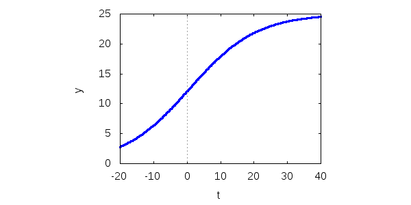
The differential equation is \[\frac{\dd y}{\dd t}=0.1\cdot y\cdot \bigl(1-0.04\cdot y\bigr)=0.1\cdot y\cdot \bigl(1-\frac{y}{25}\bigr)\] So we are dealing with a special case of the logistic equation \[\frac{\dd y}{\dd t}=r\cdot y\cdot \left(1-\frac{y}{a}\right)\] with \[r=0.1,\;a=25\] The solution of the general logistic equation is \[y(t)=\frac{a}{1+c\cdot e^{-r\cdot t}}\] for some constant \(c\). In this case we have a solution \[y(t)=\frac{25}{1+c\cdot e^{-0.1\cdot t}}\] We can calculate \(c\) by solving the equation \(y(0)=5\).

Because \(e^0=1\) we must solve \[y(0)=\frac{25}{1+c}=5\] This can be done as follows: \[\begin{aligned}\frac{25}{1+c}=5 &\stackrel{\blue{\times(1+c)}}{\implies} 25=5\cdot(1+c)\\ \\ &\stackrel{\blue{\text{expand brackets}}}{\implies} 25=5+5c\\ \\ &\stackrel{\blue{-5}}{\implies} 25-5=5c\\ \\ &\stackrel{\blue{\div 5}}{\implies} c=\frac{25-5}{5}=4\end{aligned}\] The graph for \(y(t)\) is

New example