Functions and graphs: Data and graphs
 Coordinate system
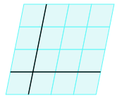
Skewed coordinate system The position of a point on a sheet of paper or on a flat surface can be indicated by means of two numbers. But for that you first have to create a coordinate system. For that you need three points, say \(O\), \(Q_1\) and \(Q_2\), that are not aligned. We choose the point \(O\) as the origin in the plane. We can use the line \(OQ_1\) as the first coordinate axis, and the line \(OQ_2\) can be used as the second coordinate axis; the origin is the intersection of these two lines. The points \(Q_1\) and \(Q_2\) can then be given the coordinates \((1,0)\) and \((0,1)\) respectively. Each point \(P\) in the plane can now be written as a point of a parallelogram with two sides along the coordinate axes, whose lengths are multiples of the lengths of the line segments \(OQ_1\) and \(OQ_2\). The scalars are the coordinates of the point \(P\). See the figure below with a skewed coordinate system.
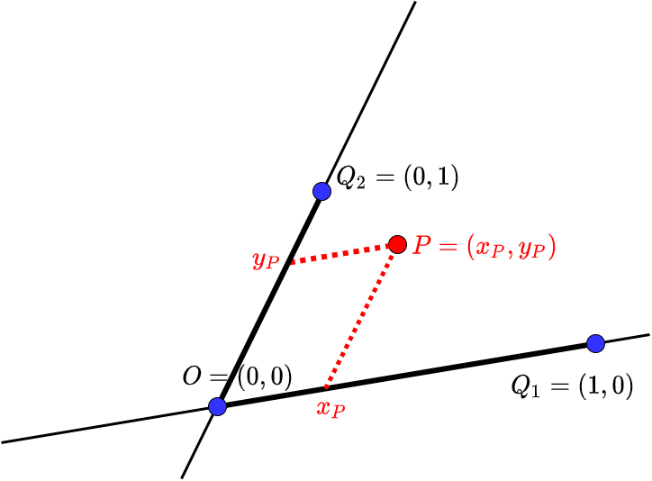
The coordinate axes in this coordinate system can be regarded as number lines and each number on a coordinate axis corresponds to a point on the axis.
Cartesian coordinate system In a rectangular coordinate system, formally called a Cartesian coordinate system, the coordinate axes are mutually perpendicular to each other and the concept of length is chosen to be equal along both axes. In the figure below two arrows are drawn in blue and red with the arrowheads ending in the points with coordinates \((1,0)\) and \((0,1)\) The points in the plane with integer coordinates together form a grid. In the figure below the grid lines are also drawn so that you get graph paper (the turquoise colouring is only for decoration).
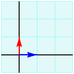
With a choice of a Cartesian coordinate system in a plane, we get a coordinate plane that we denote \(\mathbb{R}^2\).
A rectangular coordinate system with different horizontal and vertical scaling In a rectangular coordinate system you have axes in the form of number lines with the number \(0\) at the origin of the coordinate system. On the horizontal axis, the positive numbers are to the right of the origin and the negative numbers to the left; on the vertical axis, the positive numbers are above the origin and the negative numbers are below. The units, i.e., the distances between consecutive numbers, on the horizontal and vertical axes are preferably the same size, but this is not necessary. See the graph below of \(f(x)= x^5-5x^3-x^2+4x+2\) over the interval \([-2.4,2.4]\) with a vertical plot of \([-4.8,4.8]\), chosen in such a way that you get a good idea of the graph of the function.
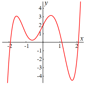
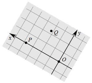
To fix the position of a point, consider how much you have to go right (or left) and up (or down) from the origin to get to that point.
Scale indications on the sides of a diagram Because the axes in a rectangular coordinate system can sometimes get in the way of a good picture of graphs, they are sometimes omitted. But then the scale indications on the sides of the diagram are visible. This also helps if the drawing region consists of very different intervals on the horizontal and vertical axes.
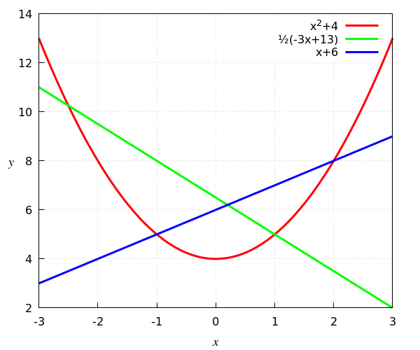
In the figure below, the graphs of the function \(x\mapsto x^2+4\), \(x\mapsto \tfrac{1}{2}(-3x+13)\) and \(x\mapsto x+6\) are drawn in one diagram. To determine the position of a point on the graph, scroll vertically down to read the \(x\) coordinate of the point on the horizontal scale and horizontally to the left to read the \(y\) coordinate of the point on the vertical scale. So you can read that in this example \((2,8)\) is a common point on the red and blue graph, i.e., is an intersection of the functions \(x\mapsto x^2+4\) and \(x\mapsto x+6\).
The figure also includes a caption at the top right that indicates which curve matches which function rule. This is called a legend to the chart.
