Basic functions: Linear functions
 Linear functions
By convention \(f\) is called a linear function (another term for first degree function) in \(x\) if the function definition can be written as \[f(x)=a\,x+b,\] for certain numbers \(a\neq 0\) and \(b\).
The graph of \(f(x)=a\,x+b\) originates from the graph of the function \(x\mapsto x\) by vertical multiplication with respect to the \(x\)-axis followed by a vertical translation.
The graph of \(f(x)=a\,x+b\) is a straight line with gradient or slope \(a\), and vertical intercept \(b\).
Below is the graph of the linear function \[C(t)=-\frac{2}{3}t+2\] in which we deliberately use variables other than the usual \(f\), \(x\), and \(y\). You can think of a concentration that decreases linearly in the course of time (for example, the blood concentration of alcohol in the human body after alcohol consumption).
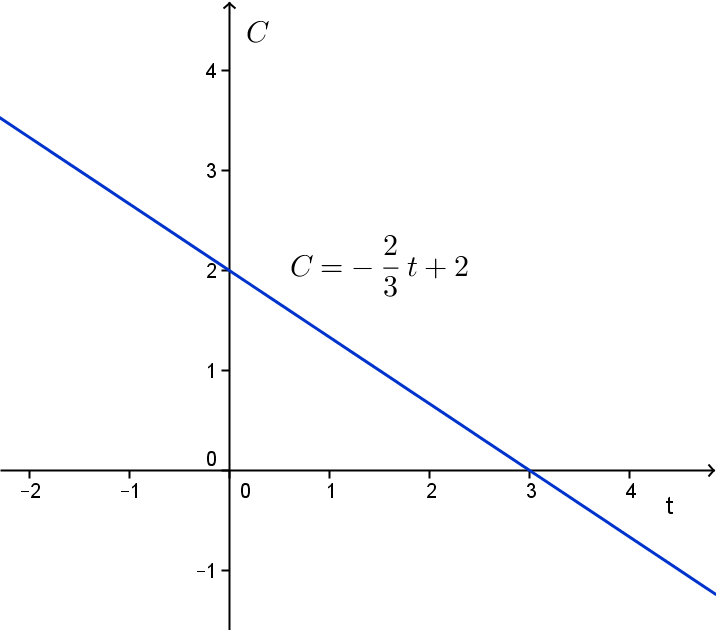
The slope can be found in the graph. The slope is in fact the ratio of the increment \({\vartriangle}C\) of \(C=C(t)\) and the increment \({\vartriangle}t\) of \(t\). For example, between \(t=0\) and \(t=3\) the increment of \(t\) is equal to \({\vartriangle}t=3-0=3\), and the increment of \(C=C(t)\) is equal to \({\vartriangle}C=0-2=-2\). The quotient is \( \displaystyle \frac{{\vartriangle}C}{{\vartriangle}t }=\frac{-2}{3}=-\frac{2}{3}\).
TThe intercept with the vertical axis can be read in this case directly in the graph because the function value at \(t=0\) is visible. If this is not the case, then you must read another point, say \((C_1,t_1)\), in the graph and calculate the intercept as \(C_1-a\cdot t_1\), under the assumption that you have already determined the slope \(a\) before.
Application in image processing An application of linear functions in image processing is a linear change in brightness and contrast by applying the function \[x\mapsto c\cdot x+b\] on the light intensity of each pixel with positive contrast parameter \(c\) (strengthening if as \(c>1\), weakening as \(0<c<1\) ) and with brightness parameter \(b\) (brighter as \(b>0\), darker as \(b<0\) ).
Linear model of a receptive field of a neuron The receptive field of visual neuron is the area in the visual field where the firing pattern changes when it is stimulated by certain visual stimuli. Assume that the response of a nerve cell to one visual image \(I_1\) is a firing pattern with frequency \(r_1=20\;\text{Hz}\) and that the response to another visual image \(I_2\) a firing pattern with frequency \(r_2=40\;\text{Hz}\). In a linear stimulus-response model, the response of this cell to the average stimuls \(\tfrac{1}{2}I_1+\tfrac{1}{2}I_2\) will be a firing pattern with frequency \(\tfrac{1}{2}r_1+\tfrac{1}{2}r_2=30\;\text{Hz}\). If one stimulus, say \(I_2\) is kept constant and the other stimulus \(I_1\) varies, we get in this model a linear function of the stimulus to the firing frequency .
Please note that this is a mathematical model only, because this model could result in an unrealistically high firing frequency in response to a strong stimulus.
Mathcentre video
Linear Functions (18:56)


