Example 1 An example of a quadratic relation is the mathematical modelling of the average height growth of girls with Turner's syndrome (a growth disorder caused by chromosomal abnormalities in which girls have retarded growth in height and no pubertal growth spurt). The average height \(L(t)\) can be modelled for age \(t\) greater than three years through the following quadratic function: \[L(t) = -0.13t^2+6.3t+70.8,\] where height \(L\) is in centimetres and age \(t\) is in years.

Example 2 The second example is a mathematical model for a population with two species; for example, think of a predator-prey system or in a microbial context of a population consisting of bacteria and immune cells. Let \(X_n\) and \(Y_n\) be the number of species X and Y in the population in year \(n\). Suppose that there is no interaction between the two species and that the population growth can be described by the following system of difference equations \[\begin{aligned} X_{n+1} &= a\cdot X_n+b\cdot Y_n\\ Y_{n+1} &= c\cdot X_n+d\cdot Y_n\end{aligned}\] for certain parameters \(a,\) \(b,\) \(c,\) \(d,\). Then, the long-term course of the population is determined by the solutions of the following quadratic equation in \(\lambda\): \[\lambda^2-(a+d)\cdot \lambda + (a\cdot d-b\cdot c) = 0\] If it is true that for the absolute values of all solutions of this equation are smaller than 1, then the population becomes extinct in the long run.

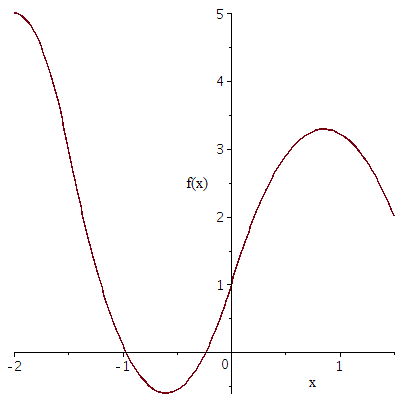
Example 3. The third example is an interpolation of function values via so-called quadratic splines. Suppose a function \(f(x)\) is defined on the interval \([-2,1.5]\) and only the following function values are known \[\begin{array}{c|c|c|c|c} x & -2 & -1.5 & 0 & 1.5 \\ \hline f(x) & 5 & 3 & 1 & 2\end{array}\] You still want to be able to calculate function values at arbitrary points in the interval \([-2, 1.5]\). This can be done by defining quadratic functions \(f_1\), \(f_2\) and \(f_3\) on the subintervals \([-2, -1.5]\), \([-1.5, 0]\) and \([0, 1.5]\) such that the function values in the edge points correspond to the function values of \(f\) (e.g., \(f_1(-1.5)=f_2(-1.5)=f(-1.5)\) ) and a smooth graph is obtained (i.e., the quadratic functions are constructed in such a way that the graphs flow neatly into each other without weird kinks at the edge points). Such functions \(f_1\), \(f_2\) and \(f_3\) on the three subintervals are called quadratic splines and can be used to calculate function values on the subintervals. In this example you can take \[\begin{aligned} f_1(x) &= -8x^2-32x-27 \\ f_2(x) &= \tfrac{40}{9}x^2+\tfrac{16}{3}x +1\\ f_3(x) &= -\tfrac{28}{9}x^2+\tfrac{16}{3}x+1\end{aligned}\] With this choice the graph of the approximation of \(f\) starts horizontally at the point \(x=-2\). This is a natural splines approximation of \(f\). See chart below for the natural splines approximation.