Applications

Exponential functions and logarithms: Exponential functions

Applications

You encounter exponential functions again and again in mathematical models of change: obviously - nomen est omen - in models of exponential growth and limited exponential growth, but also in models of logistic growth. We will study this use of exponential functions in mathematical models of growth in a later chapter, after we have gained more knowledge about these functions. Below we look at some other applications.

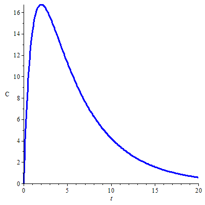
Quantitative pharmacokinetics An area of application is quantitative pharmacokinetics. For example, the course of the plasma concentration \(C(t)\) of an orally administered drug in the course of time \(t\) is often described mathematically by a bi-exponential function, with a term of absorption and one of elimination of the drug. The formula is \[C(t)=\frac{k_a A_0 F }{V_d{(k_a-k)}}\left(\e^{-k\,t}- \e^{-k_a\,t}\right).\] where \(k_a\) is the absorption rate constant, \(k\) is the elimination rate constant, \(A_0\) is the administered initial amount of the drug, \(F\) is the biological availability of the drug (i.e., the fraction of the administered drug that is comes unchanged in the general blood circulation), and \(V_d\) is the so-called volume of distribution of the drug. The mathematical formula is a bi-exponential function because it is a difference between two \(e\)-powers. The figure below shows the graph of the plasma concentration of a drug calculated with the following pharmacokinetic parameters: \[\text{oral dose}A_0=500\,\mathrm{mg},\; k_a=1.0\,\mathrm{h}^{-1},\; k=0.2\,\mathrm{h}^{-1}, \;V_d=10\,\mathrm{L}, F=0.5\,.\]

plasma concentration after oral administration of a pharmacon

Two examples of the use of the exponential function in the field of psychobiology and neuroscience:

Retention of information Hermann Ebbinghaus was one of the first psychologists who conducted quantitative research on memory. He discovered that newly learned things could be first reproduced completely, but less after some time passes. He postulated a mathematical formula for the probability that information is remembered after a certain time, the retention function \(R(t)\), by using the logarithm. However, the following exponential formula for this probability is more popular: \[R(t)=(1-R_{\infty})\cdot c\cdot \e^{-r\cdot t}+R_{\infty}\] where the term \(R_{\infty}\) reflects the fact that information is only rarely lost entirely, \(c\) is a parameter with a value between 0 and 1, and the parameter \(r\) determines the rate at which information is lost. This constant depends on many factors such as the emotional significance of the learned and the way the information is learned.

Firing of an excitable cell A Poisson process is a simple model for firing of an excitable cell (generation of an action potential). In this model, the probability \(P(k, \Delta t)\) that a cell fires \(k\) times in a time span \(\Delta t\) is given by the density \[P(k, \Delta t)=\frac{\e^{-\lambda\Delta t}(\lambda\Delta t)^k}{k!}\] Suppose the cell fires at time \(t=0\), then the probability \(p(s)\) that the cell will fire again at time \(t=s\) is according to this model equal to \[p(s)=\mu\, \e^{-\mu s}\] for \(\mu=1/\lambda\).

Finally, two examples of an exponential relationship in chemistry, and more particularly in chemical kinetics:

Arrhenius equation The reaction rate constant \(k\) for a chemical reaction often depends exponentially on the temperature \(T\) via the Arrhenius equation \[k=A\cdot \e^{-\frac{E_a}{RT}}\] where \(E_a\) is the activation energy, \(R\) is the molar gas constant, and \(A\) is a constant.

Chemical kinetics We consider two successive chemical reactions of type \[\text{A }{\mathop{\longrightarrow}\limits_{}^{k_1}} \text{ B }{\mathop{\longrightarrow}\limits_{}^{k_2}} \text{ C}\] with reaction rate constants \(k_1\) and \(k_2\). When we assume that both \(\text{A }{\mathop{\longrightarrow}\limits_{}^{k_1}} \text{ B}\) as \(\text{B }{\mathop{\longrightarrow}\limits_{}^{k_2}} \text{ C}\) are elementary reactions, then according to the law of mass action we can write down the following system of differential equations for the concentrations of A, B and C: \[ \left\{\begin{aligned} \frac{d[\text{A}]}{dt} &= -k_1\, [\text{A}] \\ \\ \frac{d[\text{B}]}{dt} &=k_1\, [\text{A}]-k_2\, [\text{B}]\\ \\ \frac{d[\text{C}]}{dt} &= k_2\, [\text{B}]\end{aligned} \right.\]

The concentrations of each substance can be calculated exacly, given the initial concentrations \([\text{A}]_0\), \([\text{B}]_0\), \([\text{C}]_0\). We examine the case \([\text{B}]_0=0, [\text{C}]_0=0\): \[ \left\{\begin{aligned} {[\text{A}]} &= [\text{A}]_0\e^{-k_1t} \\ \\ [\text{B}] &= \left\{\begin{array}{lr} [\text{A}]_0k_1\,t\,\e^{-k_1t} & \text{if }k_1=k_2 \\ \\ \dfrac{ [\text{A}]_0\,k_1}{k_2-k_1}\left(\e^{-k_1t}-\e^{-k_2t}\right) & \text{if }k_1\neq k_2 \end{array} \right. \\ \\ [\text{C}] &= [\text{A}]_0-[\text{A}]-[\text{B}]\end{aligned} \right.\]

For math enthusiasts we give a proof.

We use \(x(t)\) and \(y(t)\) for the concentrations \([\text{A}]\) and \([\text{B}]\), respectively, and we assume \([\text{A}]_0=a, [\text{B}]_0=0, [\text{C}]_0=0\). The differential equation \[\frac{dx}{dt}=-k_1\, x\] describes exponential decay and the solution equals \[x=a\,\e^{-k_1t}\] Substitution in the differential equation \(\dfrac{dy}{dt}=k_1\,x-k_2\,y\) gives \[\frac{dy}{dt}=a\,k_1\,\e^{-k_1t}-k_2\,y\] Thus:\[\frac{dy}{dt}+k_2\,y=a\,k_1\,\e^{-k_1t}\] We multiply the left- and right-hand side with \(\e^{k_2t}\) and get \[\e^{k_2t}\frac{dy}{dt}+k_2\,\e^{k_2t}\,y=a\,k_1\,\e^{(k_2-k_1)t}\] Using the calculation rules for differentiation we get: \[\frac{d}{dt}\left(\e^{k_2t}\,y\right)=a\,k_1\,\e^{(k_2-k_1)t}\] So: \[\e^{k_2t}\,y=a\,k_1\!\int \e^{(k_2-k_1)t}\,dt\] For computing the integral we distinguish two cases.

If \(k_1=k_2\), then we really have \[\e^{k_2t}\,y=a\,k_1\!\int 1\,dt\] and we get \[\e^{k_2t}\,y=a\,k_1\,t+C\] for some constant \(C\). From \(y(0)=0\) follows \(C=0\). So in this case, the solution can be written as \[y=a\,k_1\,t\,\e^{-k_1t}\]

If \(k_1\neq k_2\), then we have an exponential function as integrand. The integral can be computed and the result ist: \[\e^{k_2t}\,y=\frac{a\,k_1}{k_2-k_1}\e^{(k_2-k_1)t}+C\] From \(y(0)=0\) follows \[0=\frac{a\,k_1}{k_2-k_1}+C\] Thus: \[C= -\frac{a\,k_1}{k_2-k_1}\] So: \[\e^{k_2t}\,y=\frac{a\,k_1}{k_2-k_1}\left(\e^{(k_2-k_1)t}-1\right)\] Rewriting leads to: \[y=\frac{a\,k_1}{k_2-k_1}\left(\e^{-k_1t}-\e^{-k_2t}\right)\]

We provide a simulation to explore the successive reaction. For example, verify that if \(k_1\ll k_2\) the concentration of substance B remains low because B is rapidly converted into C, and that the kinetics differs little from that of \(\text{A}{\mathop{\longrightarrow}\limits_{}^{k_1}}\text{C}\). In contrast, \(k_2\ll k_1\) implies that a high concentration of substance B is achieved because the second reaction \(\text{B }{\mathop{\longrightarrow}\limits_{}^{k_2}}\text{ C}\) is slow, and that substance B only starts to disappears when there is almost no substance A left for conversion.