Logarithmic functions

Exponential functions and logarithms: Logarithms

Logarithmic functions

If $x$ is a positive real number, then the logarithm $\log_g(x)$ with base $g$ is defined for $g>0,\;g\neq 1$ as the real number $y$ for which the equality $g^y=x$ is valid. So:

$\log_g(x)=y\iff g^y=x$ In other words: $\log_g(x)$ is the exponent to which $g$ must be raised to obtain $x$ .
So, the equation $10^y=2$ has the solution $y=\log_{10}(2)\approx 0.301$ .

Examples

$\begin{aligned} \log_2(8)&=3&\blue{\text{because }2^3=8}\\[0.25cm]\log_3(3)&=1&\blue{\text{because }3^1=3}\\[0.25cm]\log_4(\tfrac{1}{16})&=-2&\blue{\text{because }4^{-2}=\tfrac{1}{16}}\\[0.25cm]\log_5(\sqrt{5})&=\tfrac{1}{2}&\blue{\text{because }5^{\frac{1}{2}}=\sqrt{5}}\end{aligned}$

If the base $g$ is equal to $e$ , then the logarithmic function is equal to the natural logarithm:

$\log_e(x) = \ln(x)$

For $g>0,\, g\neq 1$ we have:

$\begin{aligned} g^{\log_g(x)}&=x\quad\blue{\text{if }x>0}\\[0.25cm] \log_g(g^x)&=x\end{aligned}$

Examples

$\begin{aligned} 2^{\log_2(3)}&=3\\[0.25cm] 2^{\log_2(4)}&=4\\[0.25cm] \log_2(1)&=\log_2(2^0)=0\end{aligned}$

The logarithmic function with base $g>0,\, g\neq 1$ is defined as function $f(x)=\log_g(x)$ for positive real numbers.
The logarithmic equation $\log_g(x)=c$ has the solution $x=g^c$ . After all: $\log_g(g^c)=c$ .

Instead of $\log_g(x)$ the notation ${}^g\!\log(x)$ is also used. This notation is less convenient because it gives rise to misunderstandings sucs as interpreting $x{}^2\!\log(x)$ as $x\cdot {}^2\!\log(x)$ or as $x^2\cdot\log(x)$ .

Furthermore: $\ln(x)= \log_e(x)$ . Mathematicians often write $\log$ rather $\log_e$ or $\ln$ . Oppositely, in natural sciences $\log$ is commonly used as an abbreviation for $\log_{10}$ . SOWISO also reserves $\log$ for the logarithm with base 10. In summary, when you see $\log$ in a formula, you are advised to realize what base is used by the author.

Graphs of logarithms

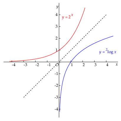
The graph of the logarithmic function can be obtained by reflection of the graph of the exponential function $f(x)=g^x$ in the line $y=x$ because these functions are each other's inverse, that is

$g^{\log_g(x)}=\log_g(g^x)=x$

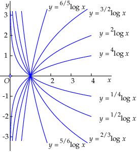
grafiek van de logartime met grondtal 2

In the figure below, the graphs of some logarithmic functions are plotted (to emphasize the base we have used the notation ${}^g\!\log(x)$ ).

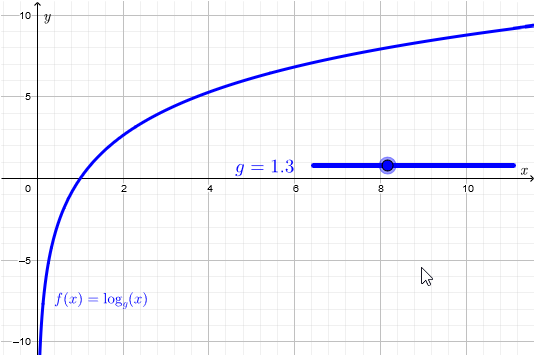
grafiek van de logartime met grondtal 2

Interactive visualisation By moving the slider in the below interactive figure below you can get an idea how the graph of the logarithmic function

$f(x)=\log_g(x)$ looks like for various values of the base $g$ .

Some properties of a logarithmic function $f(x)=\log_g(x)$ :

$f(1)=0$ (each graph of a logarithmic function passes through the point (1,0)).
$f(x)>0$ for all $x>1$ in case $g>1$ . The above graphs illustrate similar remarks.
$f$ is an increasing function if and only if $g>1$ . The larger $g$ , the less fast the function increases.
$f$ is a decreasing function if and only if $0<g<1$ . The closer $g$ is to 1, the faster the function decreases.
The vertical axis is for each logarithmic function a vertical asymptote. If $0<g<1$ , then function values $\log_g(x)$ are large for small positive $x$ (in mathematical language: $\log_g(x)\to \infty$ if $x\downarrow 0$ , or even more formal $\lim_{x\downarrow 0}\log_g(x)=\infty$ ). If $g>1$ , then $\lim_{x\downarrow 0}\log_g(x)=-\infty$ .
The function $x\mapsto x$ 'grows faster' than any multiple of a logarithmic function . In mathematical terminology: for a base $g>1$ and a natural number $n$ there exists a number $N$ such that $x>n\log_g(x)$ for all $x>N$ .

Logarithmic functions are intensively used in models of growth and, more generally, in mathematical models of processes of change, such as radioactive decay or the concentration gradient of a drug in a body. They are also used in calculations of membrane potentials.

Mathcentre videos

Logarithms (34:49)

$\phantom{x}$

Logarithmic Functions (25:48)