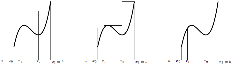
We will study several quadrature formulas for approximating the integral \(\displaystyle \int_a^b f(x)\,\dd x\) of a function \(f(x)\) over an interval \([a,b]\). We always divide the interval \([a,b]\) into \(n\) pieces by designating fixed points \(x_0, x_1, x_2,\ldots, x_n\) with \[a = x_0 < x_1 < x_2 < \cdots < x_n = b\tiny.\] in that interval. Such a set is called a partition \(V\) of \([a,b]\). We then choose a random point \(s_k\) in each sub-interval \([x_{k-1},x_k]\); we call such point a tag. So \(x_{k-1}\le s_k\le x_k\) before \(k = 1, 2, \ldots n\). The length of each of the sub-intervals \([x_{k-1},x_k]\) by \({\vartriangle}_k=x_k-x_{k-1}\) and the maximum of the lengths of the sub-intervals is called the mesh size. The expression \[R(V; s_1, \ldots, s_n)=\sum_{k=1}^nf(s_k)\cdot {\vartriangle}_k\] is called a Riemann sum corresponding with the function \(f\). Note: for a given partition \(V\) of \([a, b]\) there are many different Riemann sums: with each choice of tags you always get one. Below, for some mesh \(V\) of \([a, b]\) in which the interval is divided into three parts, three Riemann sums are given: on the left-hand side an 'arbitrary' Riemann sum, next to it the largest possible Riemann sum you can make with \(V\) (upper sum), and on the right-hand side the smallest possible Riemann sum (lower sum).

Such a Riemann sum is therefore the sum of the areas of rectangles. These rectangles together form an approximation of the area onder the curve that we want to compute. The requested area is, in a sense, a limit of such Riemann sums. A visualisation of the Riemann sums is placed below for you to play with so that you can get a better idea of the different situations (upper sum, lower sum.).

A Riemann sum is a special case of a quadrature formula, which can be written as \[K(V; s_1, \ldots, s_n)=\sum_{k=1}^nf(s_k)\cdot w_k\] for certain weights \(w_1,w_2,\ldots,w_n\). Often the tags will coincide with the points of the partition \(V\) and each weight will consist of the product of \({\vartriangle}_k\) and a sum of function values in tags and points of the partition \(V\) in the neighbourhood of the tag \(s_k\). When the tags are chosen to be equally spaced, i.e. equidistant, we speak of a Newton-Cotes quadrature formula; when the integration points are not chosen equidistant then we speak of a Gaussian quadrature formula. The latter category of quadrature formulas contains the best integration methods, but we will not discuss them.

In this chapter, a number of well-known Riemann sums and quadrature formulas will be reviewed and the task is always to implement and use the discussed method in Python in the following two cases

• \(\displaystyle \int_0^1\frac{4}{x^2+1}\,\dd x=\pi\)
  
  
• \(\displaystyle \int_0^{\pi}\sin(x)\,\dd x=2\)
  
  

We will also pay attention to the truncation errors of the different approaches.