In scientific computing, a Monte Carlo method is also popular. A Monte Carlo method is an approach to solving a mathematical problem by generating an appropriate number of randomly drawn points and determining the fraction of points with a requested property.

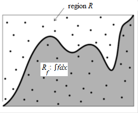
Monte Carlo integration of a function \(f(x)\) on an interval is based on calculating the area of an area under the curve—we denote this region under the curve as \(R_f\) and its area as \(\mathrm{area}(R_f)\)—via the following approach. Choose a region \(R\) that includes \(R_f\) and for which you know or can easily calculate the area \(\mathrm{area}(R)\); usually a rectangle is chosen for \(R\), but this is not necessarily the case. Now randomly generate a number of points within the region \(R\) and determine how many points are within the sub-region \(R_f\) and how many are not. You can then estimate the area of \(R_f\) as the area of the region \(R\) times the fraction of the number of points that fall within \(R_f\) in the sample.

Once the region \(R\) has been chosen, the Monte Carlo integration method boils down to the following (see the figure below):

• Take a sufficiently large uniform sample of points in the \(R\) region.
• Determine the fraction \(p\) of points that lie within the sub-region \(R_f\).
• \(\mathrm{area}(R_f)\approx p\times \mathrm{area}(R)\).

The figure above suggests that one chooses the region \(R\) as closely as possible around the \(R_f\) region. but this is not necessary. The steps of the Monte Carlo algorithm of numerically approximating \(\displaystyle \int_a^bf(x)\,\dd x\) on the interval \([a,b]\) for a nonnegative function can be written down as follows::

Step 1. Choose a rectangular region \(R\) of points \((x,y\) for which \(x_{\min}\le x\le x_{\max}\) and \(y_{\min}\le y\le y_{\max}\) with appropriately chosen \(x_{\min}, x_{\max}, y_{\min}, y_{\max}\) such that \[a\le x_{\min},\quad x_{\max}\le b,\quad y_{\min}\le f(x) \le y_{\max}\;\;\text{for all }x\text{ in }[a,b]\text.\] The basic idea is to remove from the area under the graph of \(f\) as many pieces of which you already know the surface.

Step 2. Take a sufficiently large uniform sample of points \((x,y)\) in the region \(R\). This can be done by a uniform drawing of values \(x\) from \([x_{\min},x_{\max}]\) and an equally sized uniform drawing of values \(y\) from \([y_{\min},y_{\max}]\).

Step 3. Name a point \((x,y)\) in \(R\) 'good' when \(y\le f(x)\). Note that this definition is only applicable to a positive function; with a negative function, the definition of goodness is just the opposite. The general case can also be treated, possibly by splitting the interval over which integration takes place into parts where the function is only positive or only negative. We call a point 'wrong' if it is not 'good'. In your sample, count the number of 'good' points ( \(N_\mathrm{good}\) ) and the number of 'wrong' points ( \(N_\mathrm{wrong}\) ).

Step 4. The area under the graph \(f\) within the region \(R\) is now given by \[\mathrm{opp}(R_f)=\frac{N_\mathrm{good}}{N_\mathrm{good}+N_\mathrm{wrong}}(x_{\max}-x_{\min})(y_{\max}-y_{\min})\]

Step 5. Now determine the numerical approximation of \(\displaystyle \int_a^bf(x)\,\dd x\) on the interval \([a,b]\) by adding the areas of the missing pieces to the result of the previous step.

Python task

Write your own function MonteCarloIntegral(f, a, b, sampleSize=1000) that implements the steps above.

Apply your function with a sample size of \(100\,000\) points in the following two cases:

• \(\displaystyle \int_0^1\frac{4}{x^2+1}\,\dd x=\pi\)
  
  
• \(\displaystyle \int_0^{\pi}\sin(x)\,\dd x=2\)