Numerical differentiation: Time series
 Terminology and examples
Terminology A time series or signal is defined as a quantity that usually depends on time, but may in fact depend on any other independent variable or variables. A time series is called continuous, or analogous, when observations take place continuously in time, even when the observed quantity can only take on a finite number of values (for example an on/off process). A time series is called discrete when observations are made only at specific times, usually at equal intervals. This could, for example, be the series of water levels in Vlissingen measured at fixed times per day. It may also concern data measured with a sensor over time, usually with a fixed measurement frequency ('sampling rate'). A time series can also concern calculated quantities; as an example you may think of the average daytime temperature in De Bilt, which is determined by the KNMI over time. A time series or signal is called deterministic when future values can be predicted on the basis of the observations known until then; if that is not possible, we speak of a stochastic time series.
Notation A discrete time series typically consists of a series of numbers \[y_0, y_1, y_2, y_3, \ldots \] indexed with natural numbers \(0, 1, 2, \ldots\) Each value \(y_k\) represents a measurement of a quantity \(y\) at a time \(t_k\) or an accumulation of a quantity over time intervals (for example, the number of passers-by per hour). In other words, the time series contains observations of an unknown function \(y\) of time \(t\). The function itself is mostly unknown; we only know (approximations of) function values at different times. A time series may consist of a finite or infinite number of data.
Because it is more convenient for mathematical theory formation, time series are often indexed with integers. You can extend the above time series on the left-handd side with zeros and then this time series also falls under the description \(y_n\) with integer \(n\): \[\ldots, y_{-3}, y_{-2}, y_{-1}, y_0, y_1, y_2, y_3, \ldots \] A time series can be multi-dimensional: in a 2-dimensional time series you use two indices to label the function values.
Example 1
The sinusoid with amplitude \(A\), frequency \(f\) and phase\(\varphi\), i.e., the function defined by \[y(t)=A\cdot \sin(2\pi\cdot f\cdot t+\varphi)\] is a continuous time series. The time series you get from this for \(t=\ldots -2,-1,0,1,2,\ldots\), i.e., \[y_n =A\cdot \sin(2\pi\cdot f\cdot n+\varphi)\] is an example of a discrete time series. They are drawn together in the diagram below for \(A=3, f=\tfrac{1}{6}, \varphi=\tfrac{1}{4}\pi\).

Example 2
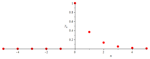
The series defined by \[y_n=\left\{\begin{array}{ll} e^{-n} & \mathrm{if\;}n=0,1,2,\ldots,\\ 0 & \mathrm{if\;}n=-1,-2,\ldots\end{array}\right.\] is a discrete time series with the following scatterplot.

Example 3
The following digital image of size \(128\times 128\) and 8-bit greyscale (between 0 and 255) is a 2-dimensional discrete signal.

It has 128 horizontal rows of 128 pixels, each of which has its own grey value from \(\{0,1,2,\ldots, 255\}\). Now two indices are needed: in the \(i\) row and \(j\) column (counting as in matrices), the function value \(g_{i,j}\) is a number from \(\{0,1,2,\ldots, 255\}\).
Time series are used in any field where only discrete values are available, such as in signal processing, pattern recognition, image processing, and control engineering.
You also want to be able to calculate derivatives for a function described in the form of a time series, calculate the area under the curve, and so on. The field that deals with the analysis of time series is called time series analysis and is also known as signal analysis. Finding a trend in measurement data is an example of such an analysis, which enables you to make predictions. But processing noise in measurements ('data smoothing') is also part of this discipline. An important part of periodic signal processing is Fourier analysis and more generally spectral analysis; we will not go into this in this course, but you may come across it in your studies.
In this chapter we mainly describe how derivatives of time series can be calculated and which methods are most suitable for this numerical differentiation.
Assumption For simplicity we will always assume that the data in a time series with fixed time steps are observed or known, i.e., the time step \(t_{k+1}-t_{k}\) is constant for all indices \(k\).


