Numerical differentiation: Time series
 Filters
In essence, a filter is nothing more than a conversion of one time series into another. Usually you use them to let pass or not pass parts of composite signals based on some criterion. For example, a sound filter can be used to reduce background noise. Another application is to filter out noise in measurement data, often referred to as 'data smoothing'.
Because numerical derivatives of measurement data are very sensitive to even small measurement errors, we take as intermezzo a look at how you can filter out such noise. We always look at a time series \(x_n\) and construct a new time series \(y_n\). We ignore edge effects for the sake of convenience.
Moving average A moving average is the average of a fixed number of consecutive elements in a time series. Usually one takes \(2q+1\) consecutive points, for some natural number \(q\) (the filter width, also called data window), around a point in the time series \(x_n\) to create a new element with the same index, for example by taking the average. Many words for the definition of the time series \(y_n\) as \[y_n=\frac{1}{2q+1}(x_{n-q}+x_{n-q-1}+\cdots x_{n+q-1}+x_{n+q})=\frac{1}{2q+1}\sum_{k=-q}^{q}x_{n+k}\tiny.\] In practice, however, the following weighted moving average is used more often \[y_n=\sum_{k=-q}^{q}\binom{2q}{k+q}\cdot (\tfrac{1}{2})^{2q}\cdot x_{n+k}\] If the filter width is \(q=2\) and \(q=1\). respectively, this means that \(y_n=\tfrac{1}{16}x_{n-2}+\tfrac{1}{4}x_{n-1}+\tfrac{3}{8}x_n+\tfrac{1}{4}x_{n+1}+ \tfrac{1}{16}x_{n+2}\) and \(y_n=\tfrac{1}{4}x_{n-1}+\tfrac{1}{2}x_n+\tfrac{1}{4}x_{n+1}\), respectively.
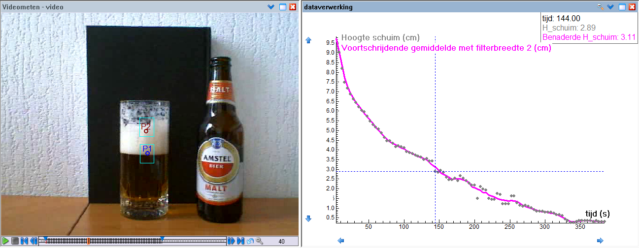
In the screen shot below you can see a video measurement of the head of a beer together with a filtering via the moving average with filter width 2. You can see that the measurement data (blue points) are somewhat smoothed (the magenta curve), or in other words, that the measurement errors are processed.


