Numerical differentiation: Time series
 Cross-correlation and convolution of time series
The moving average is an example of a linear filter created by correlation and convolution of two time series. We explain what we mean by this. But first two definitions.
Definitions If \(a_n\) and \(b_n\) are time series then the cross-correlation (or in short, correlation) of these time series, denoted as \(a\otimes b\), is defined by \[(a\otimes b)_n=\sum_k a_{n+k}b_k\]
If \(a_n\) and \(b_n\) are time series then the convolution of these time series, denoted \(a\ast b\), is defined by \[(a\ast b)_n=\sum_k a_{k}b_{n-k}\]
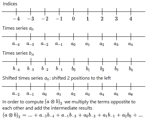
Side note: there is no unique definition of correlation and convolution in the literature. We have used the convention as implemented in for example the numpy module of the Python prgramming language. But these concepts always concern a product of a time series with another shifted time series. The visualisation below for the \(\otimes\) cross-correlation illustrates this.
We plot the time series \(a_n\) and \(b_n\) horizontally under an integer number line. As an example, we calculate \((a\otimes b)_2\).

Property The convolution operator \(\ast\) is commutative, that is \[a\ast b=b\ast a\] for time series \(a_n\) and \(b_n\).
Property The convolution operator \(\ast\) is associative, that is \[(a\ast b)\ast c=a\ast (b\ast c)\] for time series \(a_n\), \(b_n\) and \(c_n\).
A filter as cross-correlation Suppose we apply a weighted moving average with filter width\(q\) and weights \(w_k\) for \(k=-q, -q+1, \ldots q-1, q\) to a time series \(x_n\). Then we get the new time series \[y_n=\sum_{k=-q}^q x_{n+k}w_{k}\] We can extend the weights to a time series \(w_n\) by \(w_n\stackrel{\text{def}}{=}0\) for \(|n|>q\). In other words, we extend on the left-hand and right-hand side with zeros. This time series is called the kernel of the filter and the nonzero elements are called filter coefficients. Then the above sum can be rewritten as \[y_n=\sum_{k=-\infty}^{\infty} y_{n+k}w_{k}\] or in short as \[y_n=\sum_{k} y_{n+k}w_{k}\] But then we may write down that the time series \(y\) is equal to the cross-correlation of the original time series \(x\) and the kernel \(w\) of the filter. So: \[y=x \otimes w\]
A filter as convolution Given the kernel \(w\) of the linear filter, we define the adjoint of \(w\), denoted as \(w(-)\), by placing the filter coefficients backwards; in other words \[w(-)_n=w_{-n}\] for all \(n\). Then we can also write the weighted moving average as \[y_n=\sum_k y_{n+k}w_{k}=\sum_k y_{n-k}w(-)_k=\sum_k y_kw(-)_{n-k}\] But then we may write down that the time series \(y\) is equal to the convolution of the original time series \(x\) and the adjoint of \(w\). So: \[y=x \ast w(-)\]
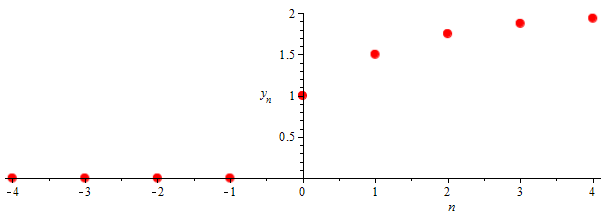
Example 1 Suppose that \(r\) is a fixed number with \(|r|<1\). We take the time series \(x\) and \(w\) defined by \[x_n=\left\{\begin{array}{ll} 1 & \text{if }n\ge 0\\ 0 & \text{if }n<0\end{array}\right.\] and \[w_n=\left\{\begin{array}{ll} 0 & \text{if }n> 0\\ r^{-n} & \text{if }n\le0\end{array}\right.\] Then we can determine the cross-correlation \(y=x\otimes w\) and the convolution \(y=x\ast w(-)\) : \[\begin{aligned}y_n& =(x \otimes w)_n= (x \ast w(-))_n=\sum_{k}x_kw(-)_{n-k}=\sum_{k}x_kw_{k-n}\\ &=\left\{\begin{array}{ll} 1+r+r^2+\cdots+r^n & \text{if }n\ge 0\\ 0 & \text{if }n<0\end{array}\right.\\ &=\left\{\begin{array}{ll} \frac{1-r^{n+1}}{1-r} & \text{if }n\ge 0\\ 0 & \text{if }n<0\end{array}\right.\end{aligned}\] The scatterplot of the filtered signal for \(r=\tfrac{1}{2}\) also suggests that the value converges for large \(n\) to \(\frac{1}{1-r}=2\):

Example 2 Calculating the results of filters can be done via computations with sparse matrices. The example below illustrates this using the weighted moving average with filter \(1\) defined by \[w_i=\left\{\begin{array}{ll} \tfrac{1}{4} & \text{if }|i|=1,\\ \tfrac{1}{2} & \text{if }i=0,\\ 0 & \text{otherwise}\end{array}\right.\] In addition to the discrete time series \(w\), we choose for the second discrete time series \(x\) the sequence defined by \[x_i=\left\{\begin{array}{ll} 2i+1 & \text{if }i=0, 1, 2, 3\\ 0 & \text{otherwise}\end{array}\right.\] The time series \(y\) resulting from cross-correlation of the time series \(x\) and \(w\) is then equal to \[y_i=(x\otimes w)_i = \left\{\begin{array}{ll} \tfrac{1}{4} & \text{if } i=-1 \\ \tfrac{5}{4} & \text{if } i=0 \\ 3 & \text{if } i=1 \\ 5 & \text{if } i=2 \\ \tfrac{19}{4} & \text{if } i=3 \\ \tfrac{7}{4} & \text{if } i=4 \\ 0 & \text{otherwise}\end{array}\right.\] This can be calculated on the basis of definitions, but also via matrix multiplication of sparse matrices (in which we take a coefficient equal to \(0\) unless explicitly defined otherwise). We write only a finite part of the time series \(x\) as a column vector and arrange the filter coefficients of \(w\) as rows along the main diagonal in a matrix such that all non-zero filtered values can be computed; in this case we do this by \[\frac{1}{4}\cdot\left(\begin{array}{cccccc} 2 & 1 & & & & \\ 1 & 2 & 1 & & & \\ & 1 & 2 & 1 & & \\ & & 1 & 2& 1 & \\ & & & 1 & 2 & 1\\ & & & & 1 & 2\end{array}\right)\cdot\left(\begin{array}{c}0\\ 1 \\ 3\\ 5\\ 7 \\ 0\end{array}\right) = \frac{1}{4}\cdot\left(\begin{array}{c}1\\5 \\ 12\\ 20\\ 19 \\ 7\end{array}\right)= \left(\begin{array}{l}0.25\\1.25 \\ 3\\ 5 \\ 4.74 \\ 1.75\end{array}\right)\]
In Python, for example, calculating with (sparse) matrices is supported in the numpy module and you can call the function correlate for this calculation via:
>>> import numpy as np
>>> np.correlate([1, 3, 5, 7], [0.25, 0.5, 0.25], "full")
array([ 0.25, 1.25, 3. , 5. , 4.75, 1.75])
In other words, you calculate with finite signals via matrix vector multiplication. With the keywords "same" or valid" instead of "full" you get for a finite input signal \(x\) an output signal \(y\) with as many values as the input signal or with fewer values, because you do not calculate edge points by adding imaginary zeros to the initial signal at the edge.
>>> np.correlate([1, 3, 5, 7], [0.25, 0.5, 0.25], "same")
array([ 1.25, 3. , 5. , 4.75])
>>> np.correlate([1, 3, 5, 7], [0.25, 0.5, 0.25], "valid")
array([ 3. , 5.])
You can calculate the convolution of two time series in Python with the convolve function. Because the chosen filter in this example is symmetrical, you get the same result:
>>> np.convolve([1, 3, 5, 7], [0.25, 0.5, 0.25], "full")
array([ 0.25, 1.25, 3. , 5. , 4.75, 1.75])


