We consider a signal \(x_n\) for \(i=1,\ldots\) and see how exponential smoothing can remove noise. We can imagine the signal \(x\) as extended with zeros for negative integer indices. It starts with convolution of this signal with the next signal which for fixed choice of \(\alpha\) between \(0\) and \(1\) is defined by \[w_n=\left\{\begin{array}{ll} \alpha (1-\alpha)^n & \mathrm{if\;}n=0,1,2,\ldots \\ 0 & \mathrm{otherwise}\end{array}\right.\] Then you may write for the convolution \(y=x\ast w\): \[y_n=\alpha x_n+ \alpha (1-\alpha)x_{n-1}+\alpha (1-\alpha)^2x_{n-2}+\cdots + \alpha (1-\alpha)^nx_0\]

1. Show that the following recurrence relation is valid for \(n>0\): \[y_n=\alpha x_n + (1-\alpha)y_{n-1}\]
2. Since \(y_0=\alpha x_0\) and \(y_n=0\) for negative \(n\), we may use this recurrence relation to calculate the convolution for each index as a weighted sum of the unfiltered value for the given index and the previous filtered value (for the given index minus 1). So we create our own convolution function and don't use a built-in function.
   
   Write a function in the selected programming language that filters a given finite signal via exponential smoothing based on the above recursion formula for a given parameter \(\alpha\). Apply your function to the beer head data from the attached excel sheet beer_head.xlsx (height of beer head versus time) or beer_head.csv (data separated by a semicolon) for three different values of \(\alpha\). Always plot the scatterplot of the measurement data and the curve after filtering in one diagram and place the three diagrams directly below each other for comparison of the smoothing achieved.
   
   Below is the graph after exponential smoothing. You can see that it takes some time for the filtered data to match the measurement data.

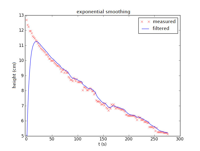
For this reason, the recurrence relation is usually not started with \(y_0=\alpha x_0\), but one takes \(y_0= x_0\) or chooses for \(y_0\) the average value of the first few measurement points. Below is the graph of filtering with a starting value chosen equal to the average of the first five measurement data

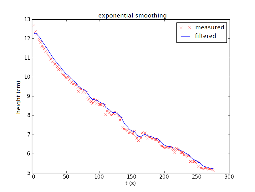
If you have the impression that the filtered graph is slightly to the right of the data plot, or in other words that the filtered data is larger than the measured data, then this may be correct. This is always the case with descending graphs because the exponential filtering tries to prevent you from running away from the values calculated up to that point. With increasing graphs you would see the opposite: then the filtered data are less than the measured data. You could make use of this by not only filtering the data in a forward direction, but also backwards starting at the last measurement data point. Below is the graph of backward filtering.

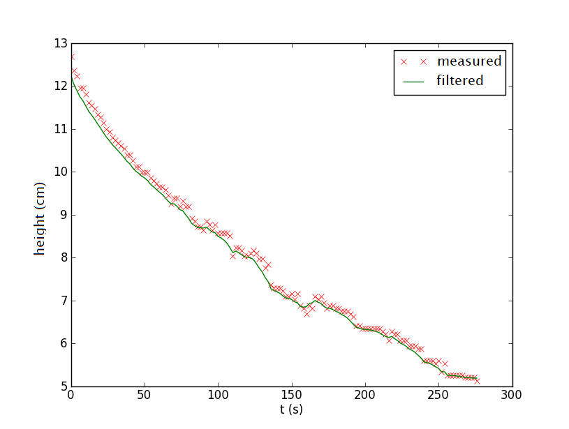
So by averaging both filtered signals you get a better result.

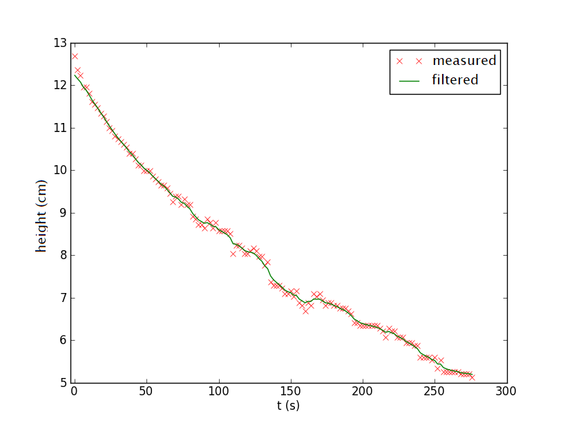
3. Implement this approach and see that you get a graph similar to this result:

4. Also try your exponential filtering function on a noisy sine graph over the interval \((0,\pi)\).