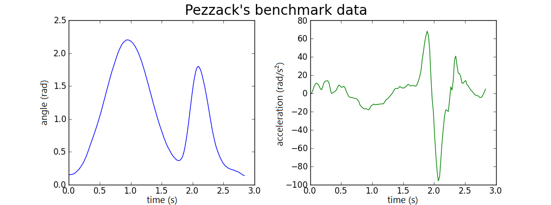
In the biomechanics literature, the following dataset Pezzack.txt from Pezzack is often used as a benchmark for data processing. It is a video measurement of a rotation of a rod in space and the angular acceleration has also been measured analogously.

The following Python code can be used to read in the data and graph the angle and acceleration

import numpy as np
import matplotlib.pyplot as plt
time, angle, angle2, a_analoog = np.loadtxt('Pezzack.txt', skiprows=6, unpack=True)
plt.figure(figsize=(11,4))
plt.suptitle("Pezzack's benchmark data", fontsize=20)
plt.subplot(1,2,1)
plt.plot(time, angle, 'b-')
plt.xlabel('time (s)', fontsize=12)
plt.ylabel('angle (rad)', fontsize=12)
plt.subplot(1,2,2)
plt.plot(time, a_analog, 'g-')
plt.xlabel('time (s)')
plt.ylabel('acceleration (rad/s$^2$)', fontsize=12)
plt.subplots_adjust(wspace=0.3)
plt.show()

In other programming languages ;ole Matlab or R you can implement the above as well.

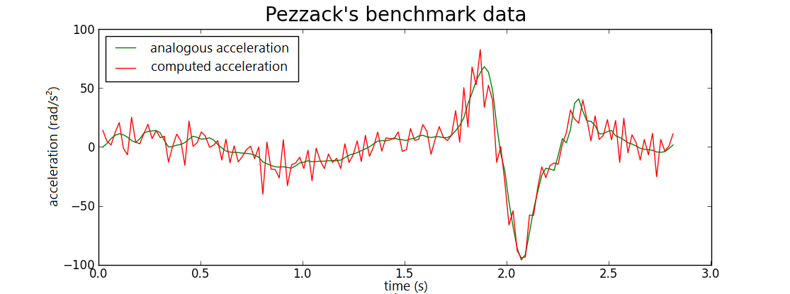
Use the 3-point central difference formula for the second derivative to approximate the acceleration numerically and plot the graph of the approximated acceleration together with the graph of the analogous measured acceleration in one figure.

If everything goes well, the diagram should look like this:

If you want better results, you myst applu more advanced methods such as Savitsky-Golay filtering or, even better, the 'cross-validatory penalized quintic spline smoothing' technique.