The bisection method, also called binary search (bisection is Latin for division in two), is a special case of a method in which the search area for a solution of a non-linear equation is systematically reduced in steps.

We start with a continuous function \(f(x)\) on the closed interval \([a,b]\) with \(f(a)\cdot f(b)<0\).
In other words, \(f(a)\) and \(f(b)\) have different signs and continuity means that you can draw the graph of \(f\) on \([a,b]\) without having to take the pen off the paper. Then the mean value theorem informs us that at least one zero of \(f\) can be found on the open interval \((a,b)\).

All we have to do is systematically reduce the interval in which we search for a zero. In the bisection method, this is done—nomen est omen—by halving repeatedly subintervals of \([a,b]\) and determining in each step which interval contains at least one zero.

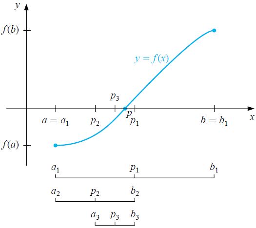
At the beginning, the interval is equal to \([a,b]\) and you first investigate whether the number \(p_1=\tfrac{a+b}{2}\) is a zero of the function \(f\). If this is the case you are done because a zero has been found; if not, split the interval into left and right subintervals, \([a,p_1]\) and \([p_1,b]\), respectively. At what interval the search for a zero continues depends on the sign of \(f(p_1)\). If this sign is opposite to that of \(f(a)\) choose the left interval, otherwise continue with the right interval. You repeat this halving process until you have reached a zero or half the length of the interval is smaller than a predetermined value. In the latter case, you choose the middle of the last found interval as an answer to an approximation of the zero of the function. The figure below illustrates the first iterations in the bisection method to find a zero\(p\) of a function \(f\).

So what you get is a sequence of intervals \[[a_1,b_1], [a_2,b_2], [a_3,b_3], \ldots\] and a sequence of approximations to a zero \[p_1, p_2, p_3, \ldots \] with \(a_1,a_2,a_3,\ldots\) an ascending sequence of numbers starting at \(a_1=a\), and \(b_1,b_2,b_3,\ldots\) a descending sequence of numbers starting at \(b_1=b\) such that \[|b_1-a_1|, |b_2-a_2|, |b_3-a_3|, \ldots\] is a strictly decreasing sequence of nonnegative real numbers. According to the above rule, we stop as soon as (coincidentally) a zero is found ( \(f(p_n)=0\) for a certain \(n\) ), or after \(n\) steps if \[\left|\frac{b_n-a_n}{2}\right|<\epsilon\] for a preselected tolerance \(\epsilon\). In other words, we stop in the bisection method when the truncation error is less than the desired accuracy.

There are, of course, other criteria for stopping to come up with.
For example, you can look at the relative truncation error \[\left|\frac{b_n-a_n}{a_n+b_n}\right|<\epsilon\] or pre-set the number of iterations \(n\) to the smallest natural number such that \[\frac{b-a}{2^n}< \epsilon\tiny.\] In the latter case you know for sure that the truncation error is less than \(\epsilon\), but if you are lucky the result will be more accurate. In any case, it is always a good idea to limit the number of iterations in a numerical algorithm: this prevents endless iteration loops.

The number of iterations required to find an answer of a certain accuracy is a measure of the method's efficiency. The speed at which the series of approximations \(p_1, p_2, \ldots\) gets closer to the zero, i.e. converges to the zero, is called the convergence speed of the method. You investigate the convergence speed by checking how many iterations are needed to find the approximation within the specified tolerance at different, ever-decreasing tolerances. Usually this is done by systematically reducing the tolerance according to a sequence \(10^{-1}, 10^{-2}, 10^{-3},\ldots \) so that more and more decimal places become correct. The convergence is linear if the relationship between the number of iterations and the number of correctly calculated decimal places is linear. This is the case in the halving method and, moreover, the truncation error halves with every iteration.

It is tempting to look at the sequence \(p_1, p_2, p_3 \ldots\) of the middles of the consecutive intervals and use one of the stopping criteria below: \[\begin{aligned} |p_n-p_{n-1}| &< \epsilon \\ \\ |f(p_n)| &< \epsilon \\ \\ \left|\frac{p_n-p_{n-1}}{p_n}\right| &< \epsilon\end{aligned}\] But each of these criteria has its problems, as we will see in exercises. For example, it is possible that a sequence \(p_1, p_2, \ldots\) has values that get closer and closer to each other without the sequence itself coming close to a fixed value. Also, small function values are no guarantee at all that you are close to a zero on the function's domain.