Linear Algebra: Linear Algebra
 Matrix Decompositions
Eigenvalue decomposition
Eigenvalue decomposition, also often called diagonalization, is a type of matrix decomposition where we utilize eigenvectors and eigenvalues. Formally, the matrix \(\mathbf{A}\) is said to be diagonalizable if we can write it in the following form: \[\mathbf{A} = \mathbf{P}\mathbf{D}\mathbf{P}^{-1},\] where \(\mathbf{D}\) is a diagonal matrix. Comparing this to change of basis equation discussed in the Change of Basis theory page, we can conclude that the columns of matrix \(\mathbf{P}\) consist of the eigenvectors (Technically, we would write \(\mathbf{D} =\mathbf{P}^{-1}\mathbf{A}\mathbf{P}\), but multiplying by both \(\mathbf{P}\) and \(\mathbf{P}^{-1}\) from both sides yields the eigendecomposition equation). This can be seen as we are switching to a basis in which our operator is diagonal, and this is exactly the basis spanned by eigenvectors.
As mentioned in the previous subsection, although it is always possible to find eigenvectors and eigenvalues for a given square matrix \(\mathbf{A}\), not every square matrix is diagonalizable. The problem here lies in the invertibility of the matrix \(\mathbf{P}\), the matrix of eigenvectors. In some cases, it can happen that the number of independent eigenvectors does not match the number of row (or columns of \(\mathbf{A}\), so the inverse \(\mathbf{P}^{-1}\) does not exist, and we cannot perform an eigenvalue decomposition.
Application of an eigenvalue decomposition In order to the usefulness of eigenvalue decomposition, let’s take a look at one use-case. Suppose that we wish to find the \(n\)-th power of the matrix \(\mathbf{A}\). Usually, we would have to perform
matrix multiplications: \[\mathbf{A}^n = \underbrace{\mathbf{A}\cdot \ldots \cdot \mathbf{A}}_{n \text{ times}}.\] However, let’s assume that the matrix \(\mathbf{A}\) is diagonalizable, so we can write it in the form \(\mathbf{A} = \mathbf{P}\mathbf{D}\mathbf{P}^{-1}\). Then, the \(n\)-th power can be calculated as follows: \[\begin{aligned} \mathbf{A}^n &= \underbrace{\mathbf{A}\cdot \ldots \cdot \mathbf{A}}_{n \text{ times}} \\[2.5mm] &= \underbrace{(\mathbf{P}\mathbf{D}\mathbf{P}^{-1})\cdot \ldots \cdot (\mathbf{P}\mathbf{D}\mathbf{P}^{-1})}_{n \text{ times}}\\[2.5mm] &= \mathbf{P}\mathbf{D}\mathbf{P}^{-1} \mathbf{P}\mathbf{D}\mathbf{P}^{-1} \cdots\mathbf{P}\mathbf{D}\mathbf{P}^{-1} \mathbf{P}\mathbf{D}\mathbf{P}^{-1} \\[2.5mm] &= \mathbf{P}\mathbf{D}^n\mathbf{P}^{-1}\\[2.5mm] \end{aligned}\] The last equation follows from the fact that \(\mathbf{P}^{-1} \mathbf{P} = \mathbf{I}\) for each intermediate term. Therefore, in this decomposition, we just need to calculate 3 matrix multiplications instead of \(n\) matrix multiplications, since the matrix \(\mathbf{D}^n\) is still a diagonal matrix whose elements are raised to the \(n\)-th power (For example if \(\lambda_i\) is the \(i\)-th diagonal element of the matrix \(\mathbf{D}\), then \(\lambda_i^n\) will be the \(i\)-th diagonal element of the matrix \(\mathbf{D}^n\).).
Singular Value Decomposition (SVD)
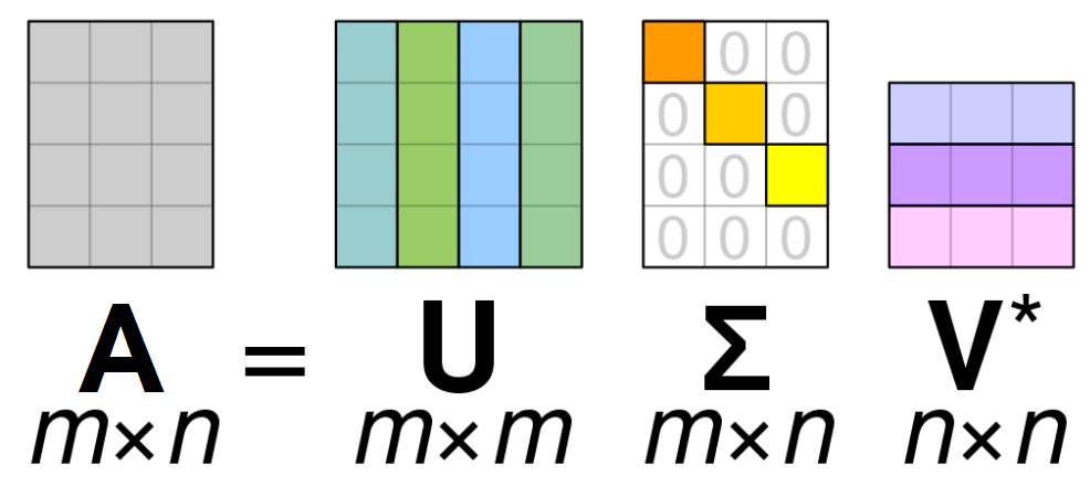
Another common type of matrix decomposition is Singular Value Decomposition, or often abbreviated as SVD. The main idea is to generalize the eigendecomposition to non-square matrices. Let’s assume that matrix \(\mathbf{A}\) is a real \(m\times n\) matrix. Then, the singular value decomposition is a factorization of the form \[\mathbf{A} = \mathbf{U}\mathbf{\Sigma}\mathbf{V}^{\top},\] where
- \(\mathbf{U}\) is an \(m\times m\) orthogonal matrix.
- \(\mathbf{\Sigma}\) is an \(m\times n\) with only nonnegative diagonal entries and for the rest zero entries.
- \(\mathbf{V}\) is an \(n\times n\) orthogonal matrix.
The visualization of these matrices is shown below (adapted from Wikipedia). We can see that the matrix \(\mathbf{\Sigma}\) has a diagonal part (which can have zero and non-zero elements), whereas the rest of the matrix is equal to zero.

The diagonal elements \(\sigma_i = \Sigma_{ii}\) of the matrix \(\mathbf{\Sigma}\) are called singular values of \(\mathbf{A}\). we can show that the number of nonzero singular values is equal to the rank of \(\mathbf{A}\). From decompositions explained in Rank of a Matrix theory page, we can see that the SVD expression is equivalent to the following: \[\mathbf{A} = \mathbf{U}\mathbf{\Sigma}\mathbf{V}^{\top} = \sum_{i=1}^{\min(m,n)} \sigma_i \cdot \mathbf{u}_i \mathbf{v}_i^{\top}\] From this, we see that the SVD of matrix \(\mathbf{A}\) expresses it as a (nonnegative) linear combination of rank-1 matrices, and we know that number of nonzero terms in such linear combination is equal to the rank of the matrix.
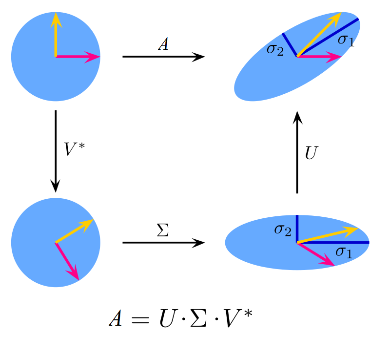
Geometrically, SVD actually performs very simple and intuitive operations. Firstly, the matrix \(\mathbf{V}\) performs a rotation in \(\mathbb{R}^n\). Next, the matrix \(\mathbf{\Sigma}\) simply rescales the rotated vectors by a singular value and appends/deletes dimensions to match the dimension \(n\) to \(m\). Finally, the matrix \(\mathbf{U}\) performs a rotation in \(\mathbb{R}^m\). In the case of a real matrix, SVD can be visualized as shown below (adapted from Wikipedia). On the top route, we can see the direct application of a matrix \(\mathbf{A}\) on two unit vectors. On the bottom route, we can see the action of each matrix in the SVD. We have used a case of a square matrix, as it is easier to visualize (in general, the matrix \(\mathbf{\Sigma}\) would add or remove dimensions, depending on the form of the matrix \(\mathbf{A}\).

Application of SVD We have motivated low-rank approximation methods in the Rank of a Matrix theory page, but we haven’t discussed how SVD can come in handy for this application. We shall first explain the procedure of using SVD for approximating matrices by their low-rank counterpart and then will show why this approach works. The rank-\(\boldsymbol{k}\) approximation \(\mathbf{A}_k\) of the matrix \(A\) can be found as follows:
- We compute the singular value decomposition of the matrix \(\mathbf{A}\) of the form \(\mathbf{A} = \mathbf{U}\mathbf{\Sigma}\mathbf{V}^{\top}\). We assume that the diagonal elements of the matrix \(\mathbf{\Sigma}\) are sorted from high to low.
- We only keep the first \(k\) columns of the matrix \(\mathbf{U}\), and we denote this matrix as \(\mathbf{U}_k\);
the shape of the matrix changes from \(m\times m\) to \(m\times k\). - We only keep the first \(k\) rows of the matrix \(\mathbf{V}^{\top}\), and we denote this matrix as \(\mathbf{V}_{k}^{\top}\); the shape of the transposed matrix changes from \(n\times n\) to \(k\times n\).
- We only keep the first \(k\) singular values (assuming they are ordered from high to low).
- The rank-\(k\) approximation \(\mathbf{A}_k\) of the matrix \(A\) is given by \(\mathbf{A}_{k}=\mathbf{U}_{k} \mathbf{\Sigma}_{k} \mathbf{V}_k^{\top}\).
Although we have found a consistent way to calculate a rank-\(k\) approximation of an arbitrary matrix, how can we know whether a low-rank approximation using SVD is any good? In order to quantify the goodness of the approximation, let’s first how we will measure it. If we treat a matrix \(\mathbf{A}\) as a vector, then the \(l_2\) norm of it (also called the Frobenius norm) is given by: \[\lVert\mathbf{A}\rVert = \sqrt{\sum_{i,j} |A_{ij}|^2}\] A good low-rank approximation \(\mathbf{A}_k\) of the matrix \(A\) can then intuitively be defined as the one that minimizes the error quantity \(\epsilon=\lVert\mathbf{A}-\mathbf{A}_k\rVert\), i.e. an approximation that will resemble the original matrix the most, measured by the Frobenius norm. In fact, it can be shown that given any rank-\(k\) matrix \(\mathbf{M}_k\) the following inequality holds: \[\lVert\mathbf{A}-\mathbf{A}_k\rVert\le \lVert\mathbf{A}-\mathbf{M}_k\rVert.\] where \(\mathbf{A_k}\) is the rank-\(k\) approximation obtained using SVD. Therefore, the low-rank approximation obtained using SVD is optimal in terms of the Frobenius norm.
Summary Eigenvalue decomposition, often called diagonalization, is a type of matrix decomposition in which we decompose a square matrix into simpler matrices that involve eigenvalues and eigenvectors. Although we can find eigenvectors and eigenvalues of all square matrices, we can diagonalize only those matrices whose eigenvectors form a basis, as we need to be able to invert the matrix that consists of eigenvectors (Only matrices whose rows are linearly independent have an inverse, i.e. have a full rank). However, we can only perform eigenvalue decomposition for square matrices which is a big limitation. In the next subsection, we will introduce singular value decomposition, which can be thought of as a generalization of the eigenvalue decomposition for non-square matrices.
The Singular Value Decomposition (SVD) breaks down a matrix into simpler components, similar to the eigendecomposition but for non-square matrices. SVD expresses a matrix as the product of three matrices: \(\mathbf{U}\), \(\mathbf{\Sigma}\), \(\mathbf{V}\). The first and third matrices are orthogonal, and the second matrix is a diagonal matrix with non-negative numbers on the diagonal called singular values. SVD allows a matrix to be expressed as a sum of simpler matrices of rank 1, and this process involves simple operations of rotation and scaling. SVD can be used to approximate a matrix by a lower-rank matrix, and the goodness of the approximation is measured by the Frobenius norm. SVD provides the best possible low-rank approximation in terms of the Frobenius norm.


