Statistics: Statistics *
 Graphical Models
Motivation Often, we know our problem at hand and wish to use independence between variables to parametrize our joint distribution efficiently. This is often done using graphical models, in which our variables form nodes in a graph and the edges from some variable to another indicate whether that first variable has ‘direct influence’ on the second. In this section, we will study one of the most common types of graphical models - the Bayesian Network - and show how using Bayesian Networks can save us many parameters needed to specify our joint.
Why graphical models?
Although this might sound surprising to many, there are a lot of statistics we can do without specifying specific distributions over our variables. Our main way to go about that is through using graphical models in which we explicitly define our variables and how they relate to each other. This allows us to formulate the (conditional) independence relationships between the variables. As seen in the previous section, knowing independent relations between the random variables can greatly reduce the number of parameters we need to learn for our joint distributions.
Getting a bit more machine learning-y, suppose we care about \(4\) different binary variables, denoted as \(X_1, X_2, X_3\), and \(Y\). For example, \(X_1, X_2, X_3\) could denote 3 different aspects of a house (e.g. \(X_1\) is many/few rooms, \(X_2\) is old/new house, and \(X_3\) one/multiple floors) and \(Y\) denotes whether it was sold for a high or low price.1 Of course, the assumption of binary variables is a little awkward here, but the intuition will be slightly easier as such. We can imagine that these \(4\) variables define one large joint distribution (of an unknown kind), i.e. for all values \(x_1, x_2, x_3\), and \(y\), we could know \(\mathbb{P}(X_1 = x_1, X_2 = x_2, X_3 = x_3, Y=y)\). It is important to realize that when we have a joint distribution, we can find any marginal or conditional probability of the variable. For example, to find the probability of the house being expensive given it has few rooms and one floor, we can find this: \[\mathbb{P}(Y = 1 \mid X_1=0, X_2 = 0) = \frac{\mathbb{P}(Y=1, X_1 = 0, X_2 = 0)}{\mathbb{P}(X_1=0, X_2 = 0)},\] which we can evaluate through marginalization by \[\mathbb{P}(Y = 1 \mid X_1=0, X_2 = 0) = \frac{\sum_{x_3} \mathbb{P}(Y=1, X_1 = 0, X_2 = 0, X_3=x_3)}{\sum_{y, x_3} \mathbb{P}(Y=y, X_1 = 0, X_2 = 0, X_3 = x_3)}.\] Having the full joint distribution is our ideal case, exactly because it allows us to ask these types of questions. In this case, we need to specify \(2^4 - 1= 15\) different values for each of the combinations of \(X_1, X_2, X_3\), and \(Y\). However, now imagine our variables taking on \(10\) different values and having \(20\) different variables. We would have to specify \(10^20\) different values. To put this into perspective, that are more values than there are grains of sand on the planet.
We will see that using graphical models and the independence relations they describe will allow us to reduce the number of parameters a lot.
Bayesian networks
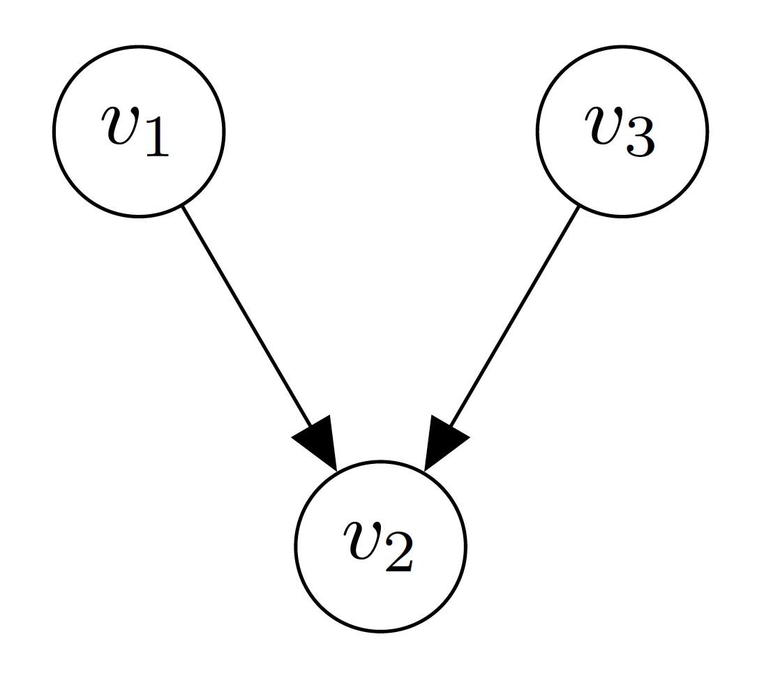
Definition A directed graph \(\mathcal{G} = (\mathcal{V}, \mathcal{E})\) is a pair of nodes (also called vertices) \(\mathcal{V}\) and edges \(\mathcal{E}\). An example of the graph with nodes \(\mathcal{V} = \{v_1, v_2, v_3 \}\) and edges \(\mathcal{E} = \{(v_1, v_2), (v_3, v_2)\}\) is visualized by

If the edges have no direction, contrary to the graph above, we call the graph undirected. If we graph is directed, there might be some path over the edges that cycles back to its starting point, in which case we call the graph cyclic. If there is no such cycle, we call the graph acyclic.
Definition A (probabilistic) graphical model is a way to express the conditional independence structures between random variables using a graph. Before diving into the formalities, let us start with an example. We will mostly focus on one type of graphical model, based on directed acyclic graphs. These models are called Bayesian networks. Do not worry if it does not all make sense in one go, it takes some time.
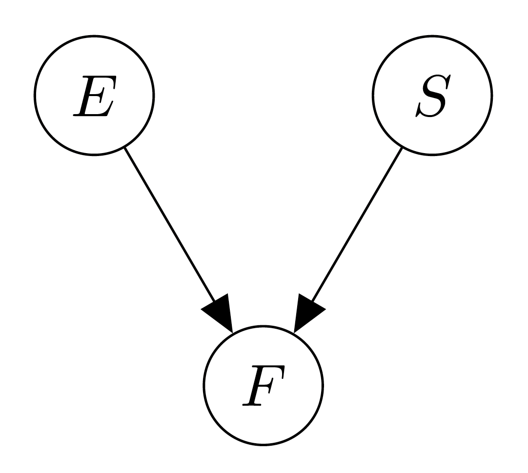
Example Suppose we revisit our espresso/strawberry story from earlier in the Indepence theory page, i.e. we have variables \(E\) for espresso, \(S\) for strawberry, and \(F\) for the lighting of fireworks. We now imagine a graph with \(3\) nodes, corresponding to these variables. The only thing missing is the edges, and we want to add an edge from \(X\) to \(Y\) if we expect there might be a direct influence of \(X\) on \(Y\). Since there is no reason to assume that the espresso I drink influences how sweet my strawberry is, we draw no arrow from \(E\) to \(S\) and visa versa. Moreover, there is a direct effect from \(E\) to \(F\), since if I drink my espresso, the fireworks will be lit. Similarly, there will be an arrow from \(S\) to \(F\). This results in the following graph:

Now, suppose we make formal what we have written above. For each node in the graph, we can consider its ‘parents’, which are all other nodes from which there exists a directed edge, i.e. for graph \(\mathcal{G} = (\mathcal{V}, \mathcal{E})\), we denote \(\mathsf{Parents}(v_i) = \{v_j \in \mathcal{V} \mid (v_j, v_i) \in \mathcal{E})\). We say that a joint distribution ‘follows’ the bayesian network if the joint distribution composes based on the parental structure in the graph. Suppose we have random variables \(X_1, \cdots, X_n\), and a graph \(\mathcal{G} = (\mathcal{V}, \mathcal{E})\) where the nodes are the \(X_i\). Then, if the joint distribution decomposes as such \[\mathbb{P}(X_1, \cdots, X_n) = \prod_{i = 1}^n \mathbb{P}(X_i \mid \mathsf{Parents}(X_i)),\] we say that the joint distribution ‘decomposes over \(\mathcal{G}\)and is a Bayesian network. So, in the case of breakfast example, we would have that \[\mathbb{P}(S, E, F) = \mathbb{P}(S) \cdot \mathbb{P}(E) \cdot \mathbb{P} (F \mid S, E).\]
Exercise Explain why in general the sparser the graph - that is, the fewer edges it has - the more parameter reduction we observe. What does this tell you about the expressivity of the joint distribution? Moreover, explain why if we add an edge from \(X\) to \(Y\) but \(X\) does not give information about \(Y\) , we are not in trouble. That is, it is OK to have too many edges, but having too few edges could harm us.
Example Let us try one more example. Suppose we have \(6\) variables, say \(X_1\) up to \(X_6\), that take on \(15\) different values. In the naive setting, we would have that \(\mathbb{P}(X_1, \cdots, X_6)\) needs \(15^6-1\approx 10^7\) values. Suppose now, that the effects are pretty simple, e.g. \(X_1\) affects directly only \(X_2\), \(X_2\) affects directly only \(X_3\), and so on. That is, our graph looks like this:

Then, we could write our joint distribution as: \[\mathbb{P}(X_1, \cdots, X_6) = \mathbb{P}(X_1) \cdot \mathbb{P}(X_2 \mid X_1) \cdot \mathbb{P}(X_3 \mid X_2) \cdot \mathbb{P}(X_4 \mid X_3) \cdot \mathbb{P}(X_5 \mid X_4)\cdot \mathbb{P}(X_6 \mid X_5).\] In this factorization, we observe that we need \(15-1=14\) parameters for the \(X_1\) distribution, and need \(15\times 15-1-224\) parameters for each of the \(\mathbb{P}(X_i \mid X_{i-1})\) distributions, i.e. a total of \(5\times 224+14=1134\) parameters rather than the ten million we started with.
Summary In this theory page, you have learned how to use independence to parametrize joints over many variables efficiently using graphical models.


