Slope field

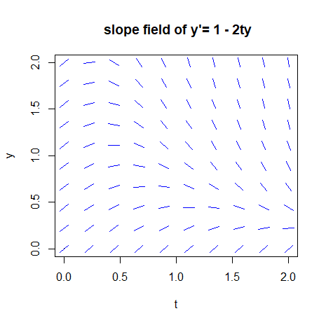
We consider the differential equation \[\frac{\dd y}{\dd t}=1-2\,t\, y\] The slope field of the above differential equation can be plotted using graphical elements such as lines.

xp <- seq(from=0, to=2, length=10)
yp <- seq(from=0, to=2, length=10)

plot(c(0,2),c(0,2), main="slope field of y'1 - 2ty", ylab = "y", xlab = "t", pch = ".")

for(x in xp){
  for(y in yp){
    u <- 1.0
    v <- 1.0 - 2.0*x*y
    L <- sqrt(u*u+v*v)
    u <- u/L
    v <- v/L
    segments(x-0.05*u,y-0.05*v,x+0.05*u,y+0.05*v, col="blue")
  }

The result is the following figure:

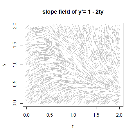
The lineal elements in the figure above are centred on a regular grid. We can also modify this program such that \(2000\) coordinates on the \(0\le t\le 2, 0\le y\le 2, \) region are randomly generated. Then, in the same way as before, we draw the lines at these coordinates. Below is an example of the R code:

xp <- runif(2000, min=0, max=2)
yp <- runif(2000, min=0, max=2)

plot(c(0,2),c(0,2), main="slope field of y'= 1 - 2ty", ylab = "y", xlab = "t", pch = ".")

for(k in 1:2000){
  x <- xp[k]
  y <- yp[k]
  u <- 1.0
  v <- 1.0 - 2.0*x*y
  L <- sqrt(u*u+v*v)
  u <- u/L
  v <- v/L
  segments(x-0.05*u,y-0.05*v,x+0.05*u,y+0.05*v, col="gray")
}

The result is now the figure below:

Just as iron filings make the field lines of a magnetic field visible, the slope field above makes the solution curves visible.

Phase portrait In this example, we consider the differential equation \[\frac{\dd y}{\dd t}=\frac{4-2t}{3y^2-5}\] solve it and draw a phase portrait.

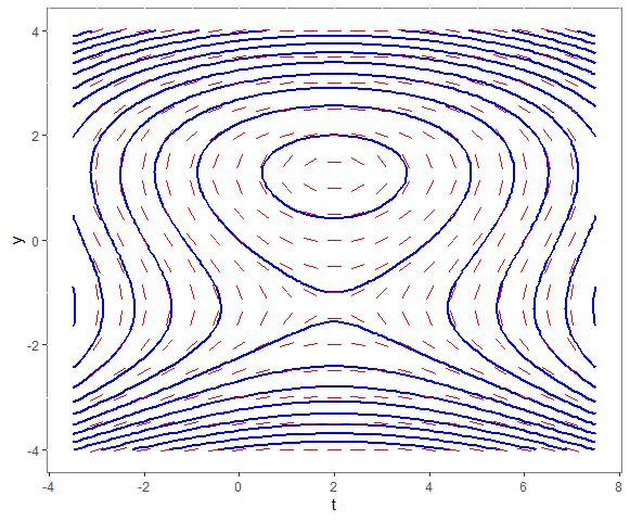
First, we write the differential equation in differential form, where we at the same time apply separation of variables: \[(3y^2-5)\,\dd y=(4-2t)\,\dd t\] If we integrate on both sides we get \[\int (3y^2-5)\,\dd y=\int (4-2t)\,\dd t\] So: \[y^3 -5y=4t-t^2+C\] for some constant \(C\). In other words \[F(t,y)=C\] for \[F(t,y)=y^3-5y+t^2-4t\]

Next, we plot a slope field and some integral curves in one diagram. The last aspect concerns contour graphing of the function \[F(t,y)=y^3-5y+t^2-4t\] The following R code, using the packages ggplot2 and dplyr, leads to the following diagram:

# load R packages
library(dplyr)
library(ggplot2)

# prepare the calculation of the slope field
tp <- seq(from=-3, to=7, by=0.5)
yp <- seq(from=-4, to=4, by=0.5)

px <- c()
py <- c()
vx <- c()
vy <- c()
for(t in tp){
  for(y in yp){
    u <- 1.0
    v <- (4.0-2.0*t)/(3.0*y^2-5.0)
    L <- sqrt(u*u+v*v)
    u <- u/L
    v <- v/L
    px <- c(px, t-0.15*u)
    py <- c(py, y-0.15*v)
    vx <- c(vx, 0.3*u)
    vy <- c(vy, 0.3*v)
  }
}
d <- data.frame(x=px, y=py, vx=vx, vy=vy)

# prepare the calculation of the contour graphs
f <- function(t,y){ y^3-5*y+t^2-4*t }
t <- seq(-3.5, 7.5, by=0.1)
y <- seq(-4, 4, by=0.1)
dat <- expand.grid(t = t, y = y) # create a grid for geom_countour
dat <- mutate(dat, z = f(t, y)) # evaluate the function at every grid point

# draw the slope field with integral curves
ggplot(dat, aes(t, y)) +
  geom_contour(aes(z = z), binwidth=6, colour="blue", size=1) +
  theme(panel.background = element_rect(fill = "white", colour = "grey50")) + 
  geom_segment(data=d, mapping=aes(x=px, y=py, xend=px+vx, yend=py+vy), colour="red") 

The integral curves describe more than one solution curve at the same time. The outer integral curve does this for 3 solution curves that depend on an initial value. We distinguish as solution curves

1. the upper part with \(y\) values greater than \(\frac{1}{3}\sqrt{15}\);
2. the middle part with \(y\) values between \(-\frac{1}{3}\sqrt{15}\) and \(\frac{1}{3}\sqrt{15}\);
3. the bottom part less than \(-\frac{1}{3}\sqrt{15}\)