Addition, scalar multiplication and linear combination You can add vectors, multiply them by a scalar, and you can combine them. This is done in the way you might expect. The only remarkable thing about addition, but what turns out to be a pleasant side effect, is that you can also add/subtract a number to a vector by considering the number as a vector of appropriate length with all values equal to the given number so that the addition/subtraction has meaning.

> u <- 1:2;  v<- 3:4
> u + v
[1] 4 6
> 5*u
[1] 5 10
> 5*u - 2*v
[1] -1 2
> u + 1
[1] 2 3

Multiplication, dot product, cross product, and the Hadamard product So far we have seen in the theory pages the inner product, the cross product and the Hadamard product. R facilitates these calculations:

> u <- 1:3; v <- 4:6 
> sum(u*v)  # standard inner product of vectors
[1] 32      
> library(pracma); dot(u,v) # alternative via pracma packge
[1] 32
> u %*% v          # alternative via matrix multiplication
    [,1]
[1,]  32
> cross(u,v)       # cross product via pracma package
[1] -3 6 -3 
array([-3, 6, -3]) 
> u*v              # Hadamard product
[1] 4 10 18

Arithmetic operations With the multiplication symbol * , you indicate that you want to apply multiplication componentwise. You can also do other arithmetic operators like division and involution. This way you can quickly construct vectors that are defined by making indexing functions or simple graphs of functions. We give some examples to illustrate

> u <- 3:4; v <- 5:6
> u / v
[1] 0.6000000 0.6666667
> u * u
[1] 9 16
> u * u
[1] 9 16
> sqrt(sum(u^2))   # computing the Euclidean length of u
[1] 5 
> i <- 1:5; v <- 1/(i+1); v # v_i = 1/(i+1)
[1] 0.5000000 0.3333333 0.2500000 0.2000000 0.1666667
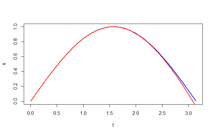
> t <- seq(0, pi, 0.01)
> s <- sin(t)
> p <- t - 1/6*t^3 + 1/120*t^5 - 1/5040*t^7;
> # display graph of sine (blue) and of a polynomial function (red)
> plot(t, s, type="l", col="blue", lwd=2)
> lines(t, p, type="l", col="red", lwd=2)  

Vectorization The previous example of a sine graph also illustrates that Python "understands" that the only meaningful use of mathematical functions on vectors is that they are used componentwise. This working style is called vectorization and makes the R language concise and clear. We give a few examples to illustrate this.

> x <- 1:5; x
[1] 1 2 3 4 5
> options(digits=4)  # format for decimal numbers
> sqrt(x)
[1] 1.000 1.414 1.732 2.000 2.236
> log(x)
[1] 0.0000 0.6931 1.0986 1.3863 1.6094
> exp(x)
[1] 2.718 7.389 20.086 54.598 148.413
> i <- 1:6; v <- (-1)^i/i; v # v_i=(-1)^i/i
[1] -1.0000 0.5000 -0.3333 0.2500 -0.2000 0.1667
> minmax <- c(min(v), max(v));  minmax  # minimum and maximum
[1] -1.0 0.5
> sum(v)     # summation of all components
[1] -0.6167
> cumsum(v)  # cummulative summation
[1] -1.0000 -0.5000 -0.8333 -0.5833 -0.7833 -0.6167
> sv <- sign(v);  sv  # signs of the components
[1] -1 1 -1 1 -1 1
> dsv <- diff(sv); dsv  # differences in consecutive signs
[1] 2 -2 2 -2 2 
> i <- (1:length(dsv))[dsv>0]; i  # indices with transition from - to + sign in v
[1] 1 3 5