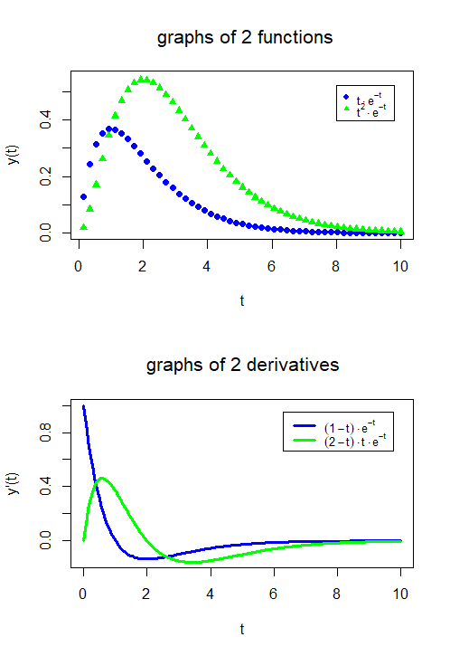
We can place graphs below or next to each other to compare them. In the following R script, the graphs of the functions \[f_1(t)=te^{-t},\quad f_2(t)=t^2e^{-t}\] are plotted in one diagram and the graphs of their first derivatives \[f_1'(t)=(1-t)te^{-t},\quad f_2'(t)=(2-t)te^{-t}\] are plotted in another diagram below. Together they form one figure. The R function that splits a figure into several parts is the following: par(mfrow=c(2,1)) fills \(2\) rows and \(1\) column with graphs. This time we have put the formulas in the legend in a more mathematical notation via the expression function.

# define the functions and their derivatives
f1  <- function(t) { t * exp(-t) }
f2  <- function(t) { t^2 * exp(-t) }
f1p <- function(t) { (1-t) * exp(-t) }
f2p <- function(t) { (2-t) * t * exp(-t) }

# create time intervals and function values
t <- seq(from=0, to=10, length=204)
tt <- t[seq(from=0, to=204, by=4)]
y1 <- f1(tt)
y2 <- f2(tt)
y1p <- f1p(t)
y2p <- f2p(t)

par(mfrow=c(2,1)) # 2 diagrams below each other

# upper diagram with graphs of functions
plot(tt, y1, type="p", col="blue", pch=16, lwd=3, ylim=c(0,0.55),
  main="graphs of 2 functions", xlab="t", ylab="y(t)")
  points(tt, y2, type="p", col="green", pch=17, lwd=3)
  legend(8, 0.52, text.width=1,
  legend=expression(t%.%e^-t,t^2%.%e^-t),
  col=c("blue", "green"), pch=c(16,17), cex=0.8)
 # lower diagram with graphs of derivatives
 plot(t, y1p, type="l", col="blue", lwd=3, ylim=c(-0.15,1),
   main="graphs of 2 derivatives",
   xlab="t", ylab="y'(t)")
   lines(t, y2p, type="l", col="green", lwd=3)
   legend(6.3, 0.95, text.width=2,
   legend=expression((1-t)%.%e^-t, (2-t)%.%t%.%e^-t),
   col=c("blue", "green"), lwd=3, cex=0.8)

The result looks like this: