Regression analysis involves establishing a relationship between a dependent variable \(y\) and one or more independent variables. We limit ourselves here to linear regression analysis in one variable, that is, to find a linear relationship \[y=\beta_0+\beta_1x\tiny,\] where \(x\) is the independent variable, and \(\beta_0\) and \(\beta_1\) are parameters to be estimated such that the straight line best fits measurement data. This line is called the regression line and the corresponding equation is referred to as the regression equation or regression model.

When estimating the parameters in the regression equation, we distinguish between the measured data \((x_1,y_1), \ldots, (x_n,y_n)\) and the estimated values \((x_1,\hat{y}_1), \ldots, (x_n,\hat{y}_n)\) recorded by \[\hat{y}_i=\beta_0+\beta_1x_i\tiny.\] In the least squares method, values of \(\beta_0\) and \(\beta_1\) are calculated such that the sum of the squared deviations is minimal. In other words, we then give ourselves the following task \[\text{Minimise }\sum_{i=1}^n(y_i-\hat{y}_i)^2\] The result is as follows: \[\begin{aligned} \beta_1 &= \frac{\displaystyle\sum_{i=1}^n (x_i-\bar{x}) (y_i-\bar{y})}{\displaystyle\sum_{i=1}^n (x_i-\bar{x})^2}\\ \\ \beta_0 &= \bar{y}-\beta_1\bar{x}\end{aligned}\] with \[\bar{x}=\frac{1}{n}\sum_{i=1}^nx_i,\quad\text{and}\quad \bar{y}=\frac{1}{n}\sum_{i=1}^ny_i\] The difference between a measured and an estimated value, say \(\epsilon_i=y_i-\hat{y}_i\), is called a residual value (or residual in short). The residuals say something about the quality of the regression line with regards to the slope. The mean squared deviation, defined as \(\displaystyle \frac{1}{n-2}\sum_{i=1}^n \epsilon_i^2\), is a measure of the quality of the regression model. In this case, the (residual) standard deviation is usually chosen, which is defined as the square root of the mean squared deviation. The standard deviation of the slope estimation is \[\begin{aligned}\text{sd}(\beta_1) &= \sqrt{\dfrac{1}{n-1}\displaystyle\sum_{i=1}^n \epsilon_i^2}\\[0.25cm] &=\frac{1}{\sqrt{n-1}} \sqrt{\displaystyle\sum_{i=1}^n(y_i-\beta_0-\beta_1x_i)^2}\end{aligned}\] You can also calculate the correlation coefficient between the measured and estimated values as an indication of the quality of the model.

Linear regression by a straight line is easily done in R with the lm instruction (linear model). The following example illustrates this.

x <- seq(from=0, to=20, by=1)
y <- runif(1, min=1, max=10)+ runif(1, min=0, max=5)*x + 
  rnorm(21, mean=0, sd=1)

# lineaire regression by  straight line
fit <- lm(formula = y ~ x)
print(summary(fit))
# correlation between given data and data generated by linear fit
cat("correlation coefficient =", cor(y,predict(fit)))

# Visualisation of data + regression line
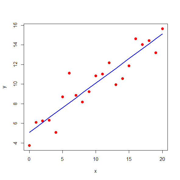
plot(x, y, type = "p", pch = 16, col = "red", cex = 1.3)
lines(x, predict(fit), type="l", col="blue", lwd=2)

Call:
lm(formula = y ~ x)

Residuals:
    Min      1Q  Median      3Q     Max 
-2.0006 -0.9072  0.2761  0.5443  3.0466 

Coefficients:
            Estimate Std. Error t value Pr(>|t|)    
(Intercept)  5.07152    0.53114   9.548 1.10e-08 ***
x            0.50248    0.04543  11.060 1.01e-09 ***
---
Signif. codes:  0 ‘***’ 0.001 ‘**’ 0.01 ‘*’ 0.05 ‘.’ 0.1 ‘ ’ 1

Residual standard error: 1.261 on 19 degrees of freedom
Multiple R-squared:  0.8656,	Adjusted R-squared:  0.8585 
F-statistic: 122.3 on 1 and 19 DF,  p-value: 1.015e-09

correlatie coefficient = 0.9303508